Autoplot and autolayer methods for multivariate (tf_mv) objects

Plotting methods for vector-valued functional data (tf_mv, functions \(R \to R^d\)), mirroring the display modes of tf::plot.tf_mv().

Usage

# S3 method for class 'tf_mv'
autoplot(object, ..., type = NULL, colour_by_arg = FALSE)

# S3 method for class 'tf_mv'
autolayer(object, ..., type = NULL, colour_by_arg = FALSE)

Arguments

object

a tf_mv object

...

passed to geom_path() (trajectory) or geom_line() (facet)

type

"trajectory", "facet", or NULL to resolve from the number of components (see Details).

colour_by_arg

colour the segments of trajectories by their argument value? Defaults to FALSE. Only available for type = "trajectory".

Value

A tf_ggplot() object for autoplot(), a ggplot2::layer() for autolayer().

Details

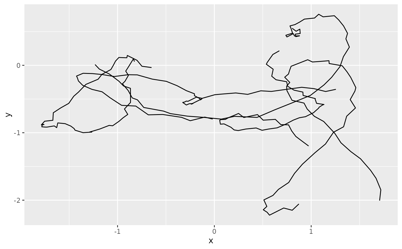
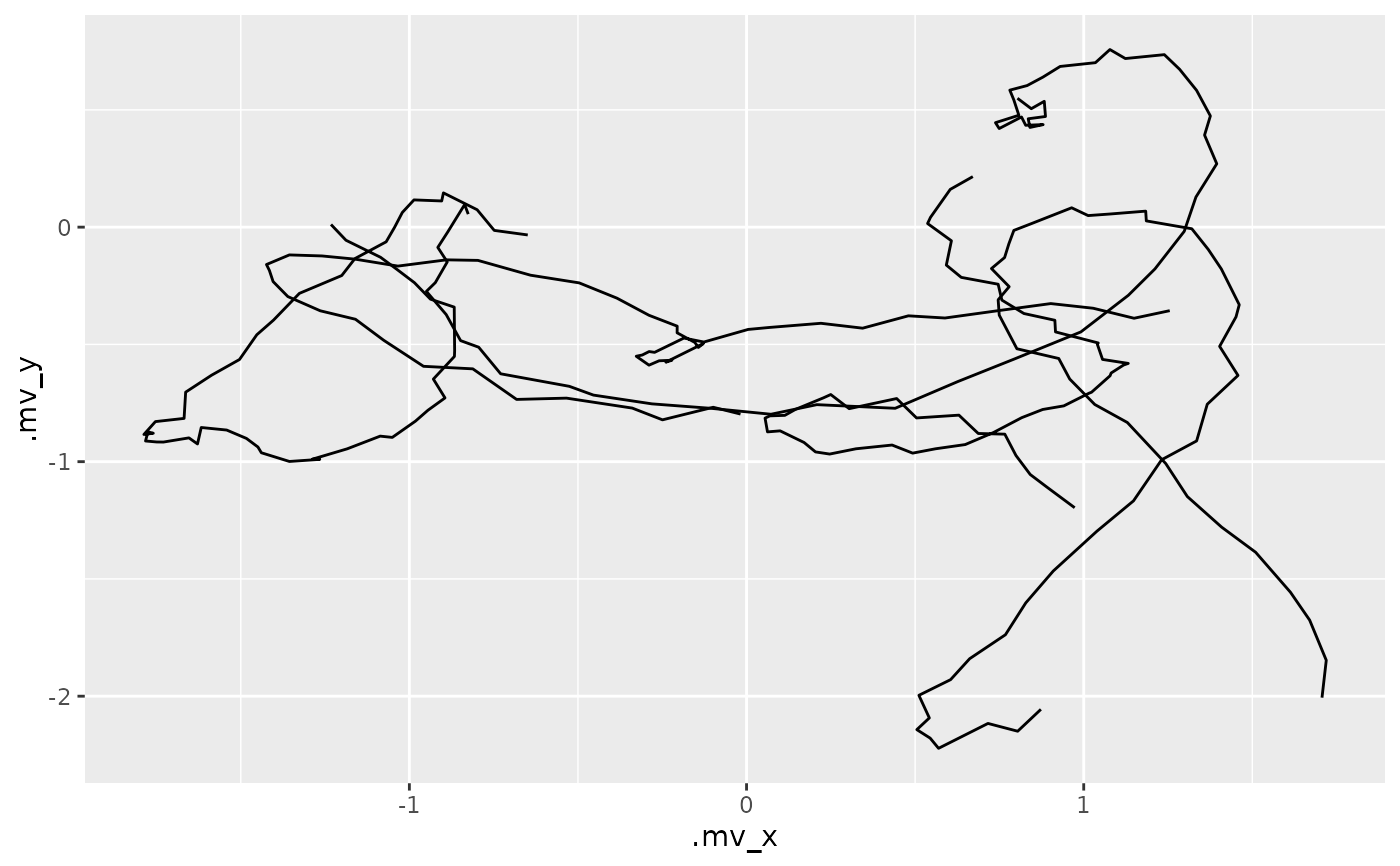
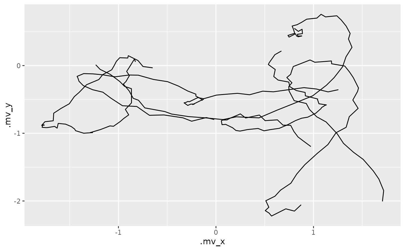
For two-component objects (d == 2) the default is a "trajectory" plot of the planar curve x(t) vs y(t) (drawn with geom_path(), which connects in argument order). Otherwise the default is "facet": value-vs-arg curves with one panel per output dimension. autolayer() returns a single layer (no faceting) and works with plain ggplot2::ggplot() as well as tf_ggplot().

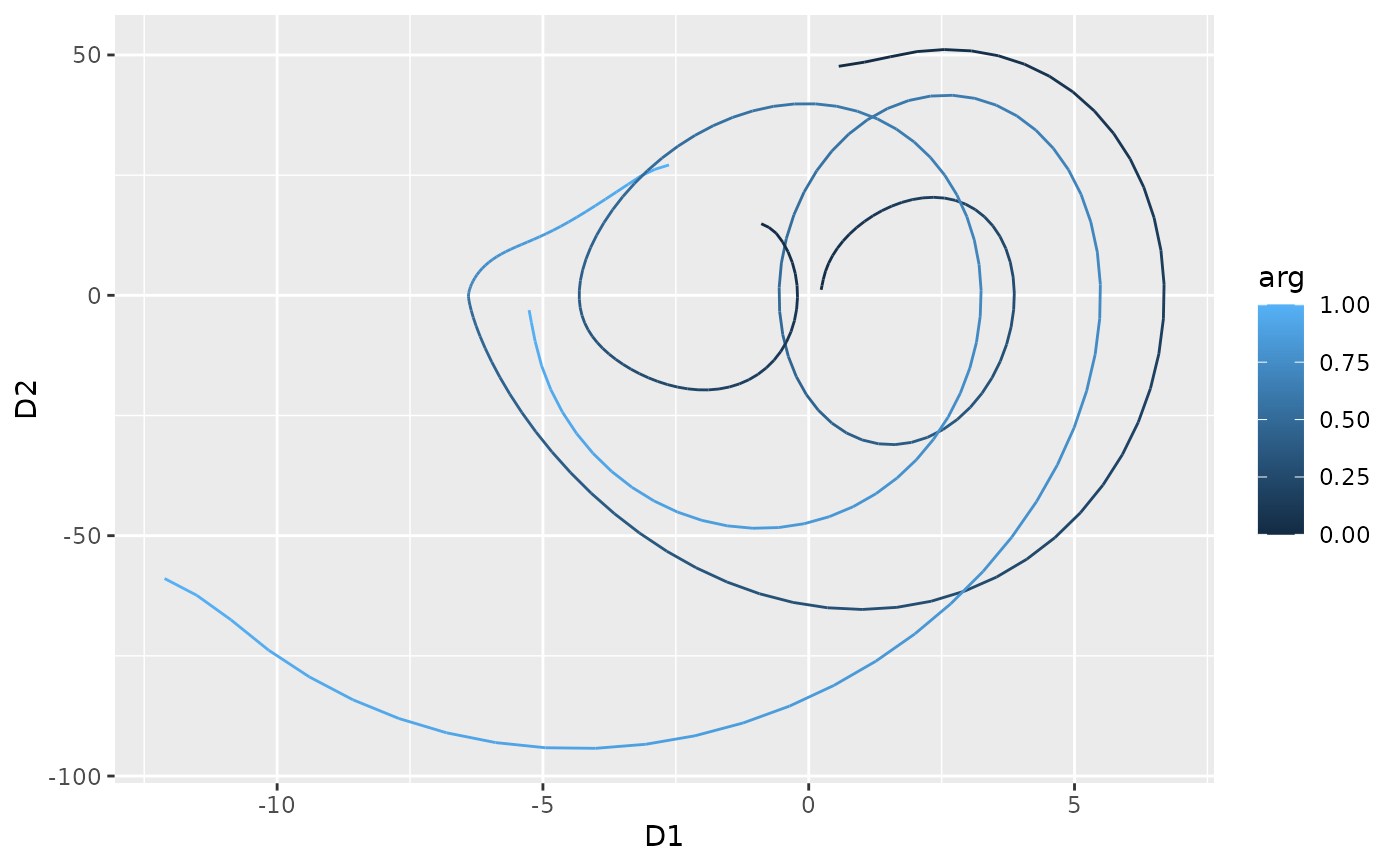
Trajectory plots lose the information about where along the domain a point lies. Set colour_by_arg = TRUE to colour each segment of the trajectories by its argument value. This maps the .arg column that tf_ggplot() provides to the colour aesthetic, so autoplot(mv, colour_by_arg = TRUE) is equivalent to tf_ggplot(data, aes(tf = mv, colour = .arg)) + geom_path().

See also

tf_phaseplane() for phase-plane plots of univariate functions.

Other tidyfun visualization: autoplot.tf(), ggcapellini, gglasagna(), ggspaghetti, tf_phaseplane()

Examples

library(ggplot2)
mv <- tfd_mv(list(x = tf_rgp(5), y = tf_rgp(5)))
autoplot(mv)

autoplot(mv, colour_by_arg = TRUE)

ggplot() + autolayer(mv)

# phase-plane plot of a univariate function (velocity vs. acceleration):
f <- tf_rgp(3, arg = 101L, nugget = 0)
autoplot(tf_phaseplane(f), colour_by_arg = TRUE)