Phase-plane representation of functional data

Turns a univariate tf vector into a two-component tf::tfd_mv() / tf::tfb_mv() object holding two derivatives of each function, so that the curves can be displayed as trajectories in the plane spanned by these derivatives – a phase-plane plot like fda::phaseplanePlot(). By default, the first derivative (velocity, on the horizontal axis) is paired with the second derivative (acceleration, on the vertical axis). 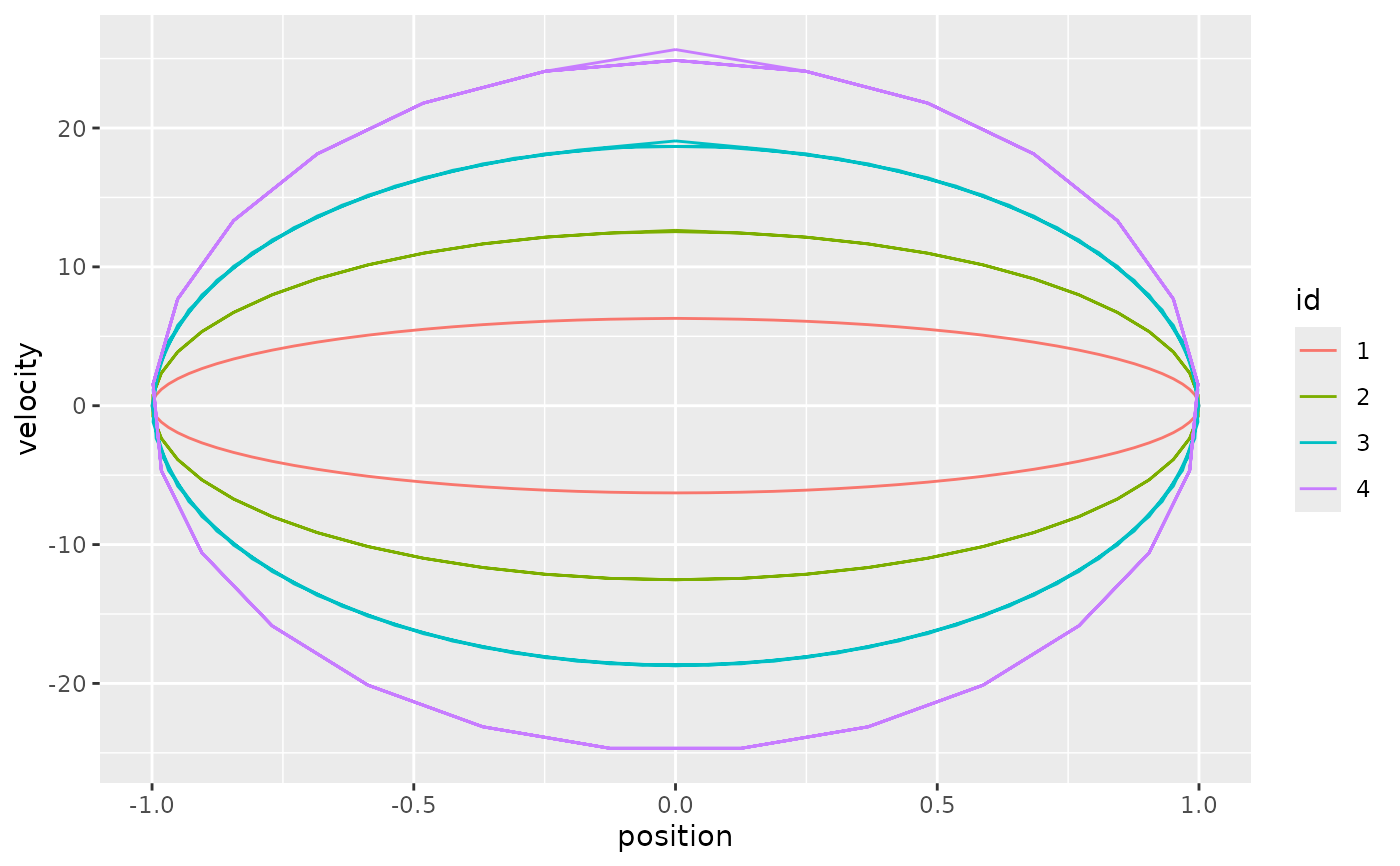Use order = c(0, 1) for the classical phase portrait of position vs. velocity.

Usage

tf_phaseplane(f, order = c(1L, 2L), arg = NULL)

Arguments

f: a univariate tf object (tfd or tfb)
order: integer vector of length 2: the derivative orders shown on the x- and y-axis. Defaults to c(1, 2) (velocity vs. acceleration); 0 means the function itself. Maximal order for tf::tfb_spline() objects is 2.
arg: optional grid on which to evaluate the derivatives (and, for order 0, the function itself); defaults to f's own grid, see tf::tf_derive().

Value

A two-component tf_mv object (tfb_mv for tfb input if both components can be represented in basis form and no arg is given, otherwise tfd_mv) with components named "D<order>", e.g. "D1" and "D2".

Details

Derivatives are computed with tf::tf_derive(), i.e. by finite differences for tfd objects. Since differencing amplifies noise, phase-plane plots of raw data are usually only informative for smooth functions (e.g. a tf::tfb() representation, or tf::tf_smooth()ed data) on a fine grid.

The result is a regular tf_mv object, so it can be plotted with tf_ggplot() (map it with aes(tf = ...) and add ggplot2::geom_path()) or autoplot(). Use aes(colour = .arg) or colour_by_arg = TRUE to colour the trajectories by their argument value, which is otherwise not visible in a phase-plane plot.

Examples

library(ggplot2)
arg <- seq(0, 1, length.out = 101)
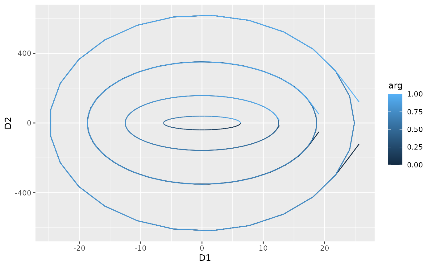
# sinusoids of varying frequency: the phase plane shows nested ellipses
f <- tfd(t(sapply(1:4, \(k) sin(2 * pi * k * arg))), arg = arg)
pp <- tf_phaseplane(f)
pp
#> tfd_mv<d=2>[4] (D1, D2): [0, 1] -> [-24.67289, 25.65029] x [-617.2462, 617.2462]
#> components based on 101 evaluations each, interpolation by tf_approx_linear
#> [1]: ▅▅▅▅▅▅▄▄▄▄▄▃▃▃▃▄▄▄▄▄▅▅▅▅▅▅ | ▄▄▄▄▄▄▄▄▄▄▄▄▄▅▅▅▅▅▅▅▅▅▅▅▅▅
#> [2]: ▆▆▅▄▃▃▂▃▃▄▅▆▆▆▆▅▄▃▃▂▃▃▄▅▆▆ | ▄▄▄▄▄▄▄▅▅▆▅▅▅▄▄▄▄▄▄▅▅▅▆▅▅▅
#> [3]: ▇▆▄▂▂▂▄▆▇▇▅▃▂▂▃▅▇▇▆▄▂▂▂▄▆▇ | ▄▃▂▃▅▆▇▆▅▃▂▃▄▅▆▇▆▄▃▂▃▄▆▇▆▅
#> [4]: █▅▂▁▃▆█▇▃▁▂▅██▅▂▁▃▇█▆▃▁▂▅█ | ▃▁▂▅██▅▂▁▄▇█▆▃▁▂▅█▇▄▁▁▄▇█▆
#> 
autoplot(pp, colour_by_arg = TRUE)

# position vs. velocity, with tf_ggplot:
d <- data.frame(id = factor(1:4))
d$f <- f
tf_ggplot(d, aes(tf = tf_phaseplane(f, order = c(0, 1)), colour = id)) +
  geom_path() +
  labs(x = "position", y = "velocity")