Converting to & from `tf`

Functional data have often been stored in matrices or data frames. Although these structures have sufficed for some purposes, they are cumbersome or impossible to use with modern tools for data wrangling.

In this vignette, we illustrate how to convert data from common structures to tf objects. Throughout, functional data vectors are stored as columns in a data frame to facilitate subsequent wrangling and analysis.

Conversion from matrices

One of the most common structures for storing functional data has been a matrix. Especially when subjects are observed over the same (regular or irregular) grid, it is natural to observations on a subject in rows (or columns) of a matrix. Matrices, however, are difficult to wrangle along with data in a data frame, leading to confusing and easy-to-break subsetting across several objects.

In the following examples, we’ll use tfd to get a tf vector from matrices. The tfd function expects data to be organized so that each row is the functional observation for a single subject. It’s possible to focus only on the resulting tf vector, but in keeping with the broader goals of tidyfun we’ll add these as columns to a data frame.

The DTI data in the refund package has been a popular example in functional data analysis. In the code below, we create a data frame (or tibble) containing scalar covariates, and then add columns for the cca and rcst track profiles. This code was used to create the tidyfun::dti_df dataset included in the package.

dti_df <- tibble(
  id = refund::DTI$ID,
  visit = refund::DTI$visit,
  sex = refund::DTI$sex,
  case = factor(ifelse(refund::DTI$case, "MS", "control"))
)

dti_df$cca <- tfd(refund::DTI$cca, arg = seq(0, 1, length.out = 93))
dti_df$rcst <- tfd(refund::DTI$rcst, arg = seq(0, 1, length.out = 55))

In tfd, the first argument is a matrix; arg defines the grid over which functions are observed. The output of tfd is a vector, which we include in the dti_df data frame.

dti_df
## # A tibble: 382 × 6
##       id visit sex    case                                            cca
##    <dbl> <int> <fct>  <fct>                                   <tfd_irreg>
##  1  1001     1 female control (0.000,0.49);(0.011,0.52);(0.022,0.54); ...
##  2  1002     1 female control (0.000,0.47);(0.011,0.49);(0.022,0.50); ...
##  3  1003     1 male   control (0.000,0.50);(0.011,0.51);(0.022,0.54); ...
##  4  1004     1 male   control (0.000,0.40);(0.011,0.42);(0.022,0.44); ...
##  5  1005     1 male   control (0.000,0.40);(0.011,0.41);(0.022,0.40); ...
##  6  1006     1 male   control (0.000,0.45);(0.011,0.45);(0.022,0.46); ...
##  7  1007     1 male   control (0.000,0.55);(0.011,0.56);(0.022,0.56); ...
##  8  1008     1 male   control (0.000,0.45);(0.011,0.48);(0.022,0.50); ...
##  9  1009     1 male   control (0.000,0.50);(0.011,0.51);(0.022,0.52); ...
## 10  1010     1 male   control (0.000,0.46);(0.011,0.47);(0.022,0.48); ...
## # ℹ 372 more rows
## # ℹ 1 more variable: rcst <tfd_irreg>

Finally, we’ll make a quick spaghetti plot to illustrate that the complete functional data is included in each tf column.

dti_df |>
  tf_ggplot(aes(tf = cca, col = case, alpha = 0.2 + 0.4 * (case == "control"))) +
  geom_line() +
  facet_wrap(~sex) +
  scale_alpha(guide = "none", range = c(0.2, 0.4))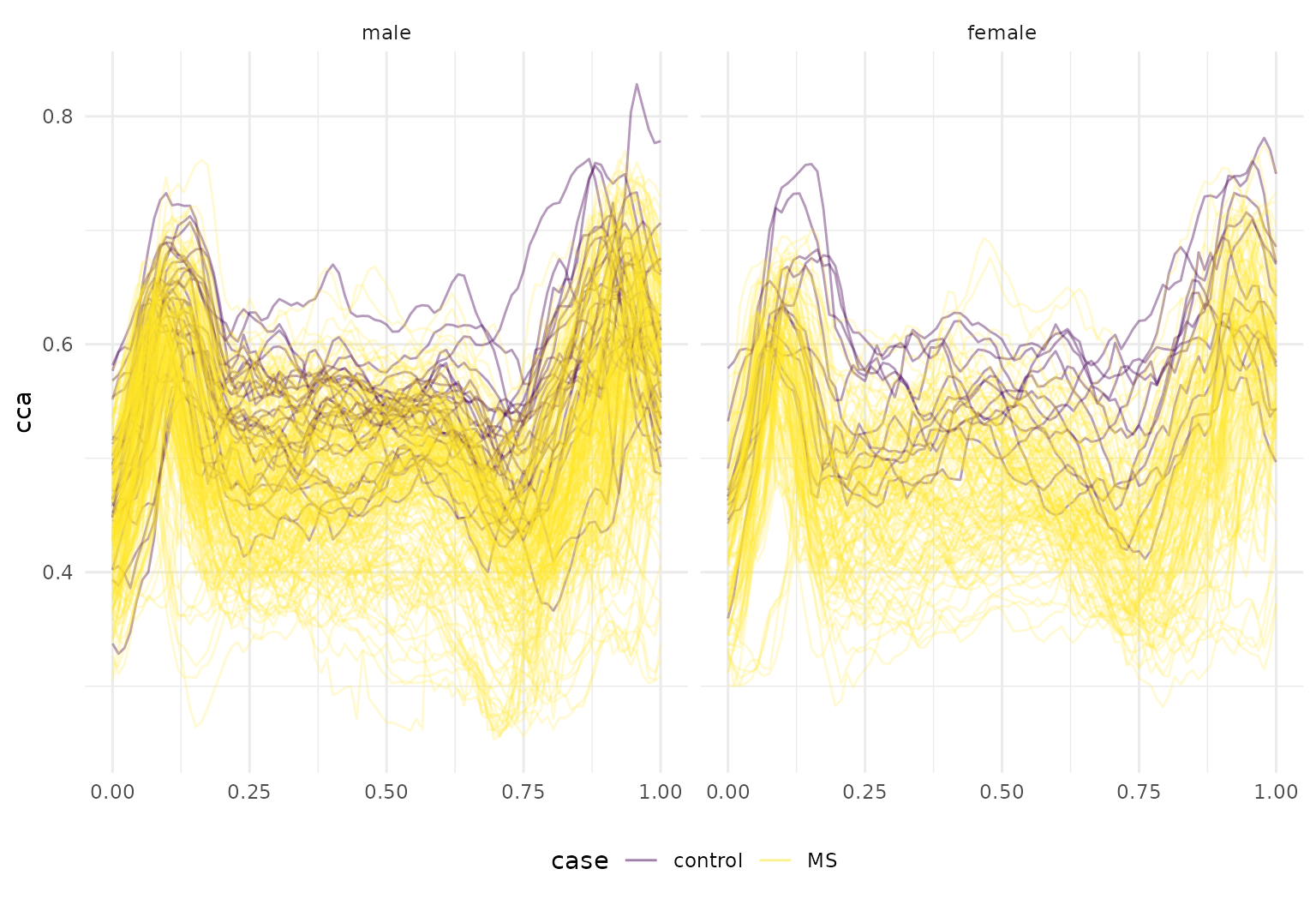

We’ll repeat the same basic process using a second, and probably even-more-perennial, functional data example: the Canadian weather data in the fda package. Here, functional data are stored in a three-dimensional array, with dimensions corresponding to day, station, and outcome (temperature, precipitation, and log10 precipitation).

In the following, we first create a tibble with scalar covariates, then use tfd to create functional data vectors, and finally include the resulting vectors in the dataframe. In this case, our args are days of the year, and we use tf_smooth to smooth the precipitation outcome. Because the original data matrices record the different observations in the columns instead of the rows, we have to use their transpose in the call to tfd:

canada <- tibble(
  place = fda::CanadianWeather$place,
  region = fda::CanadianWeather$region,
  lat = fda::CanadianWeather$coordinates[, 1],
  lon = -fda::CanadianWeather$coordinates[, 2]
) |>
  mutate(
    temp = t(fda::CanadianWeather$dailyAv[, , 1]) |>
      tfd(arg = 1:365),
    precipl10 = t(fda::CanadianWeather$dailyAv[, , 3]) |>
      tfd(arg = 1:365) |>
      tf_smooth()
  )
## Using `f = 0.15` as smoother span for `lowess()`.

The resulting data frame is shown below.

canada
## # A tibble: 35 × 6
##    place       region     lat   lon                       temp
##    <chr>       <chr>    <dbl> <dbl>                  <tfd_reg>
##  1 St. Johns   Atlantic  47.3 -52.4 ▄▄▄▄▄▅▅▅▆▆▆▇▇▇██▇▇▇▇▆▆▆▅▅▅
##  2 Halifax     Atlantic  44.4 -63.4 ▄▄▄▄▄▅▅▆▆▇▇▇██████▇▇▆▆▆▅▅▄
##  3 Sydney      Atlantic  46.1 -60.1 ▄▄▄▄▄▅▅▅▆▆▇▇██████▇▇▆▆▆▅▅▄
##  4 Yarmouth    Atlantic  43.5 -66.1 ▄▄▄▄▅▅▅▆▆▇▇▇▇█████▇▇▇▆▆▆▅▅
##  5 Charlottvl  Atlantic  42.5 -80.2 ▄▄▃▄▄▄▅▅▆▆▇▇██████▇▇▆▆▆▅▄▄
##  6 Fredericton Atlantic  45.6 -66.4 ▃▃▃▄▄▅▅▆▆▇▇███████▇▇▆▆▅▅▄▄
##  7 Scheffervll Atlantic  54.5 -64.5 ▁▁▁▁▂▂▃▄▄▅▆▆▇▇▇▇▇▆▆▅▅▄▄▃▂▁
##  8 Arvida      Atlantic  48.3 -71.1 ▂▂▂▃▃▄▅▆▆▇▇███████▇▆▆▆▅▄▃▃
##  9 Bagottville Atlantic  48.2 -70.5 ▂▂▂▃▃▄▅▅▆▇▇▇█████▇▇▆▆▅▅▄▃▃
## 10 Quebec      Atlantic  46.5 -71.1 ▃▃▃▃▄▄▅▆▆▇▇███████▇▇▆▆▅▄▄▃
## # ℹ 25 more rows
## # ℹ 1 more variable: precipl10 <tfd_reg>

A plot containing both functional observations is shown below.

temp_panel <- canada |>
  tf_ggplot(aes(tf = temp, color = region)) +
  geom_line()

precip_panel <- canada |>
  tf_ggplot(aes(tf = precipl10, color = region)) +
  geom_line()

gridExtra::grid.arrange(temp_panel, precip_panel, nrow = 1)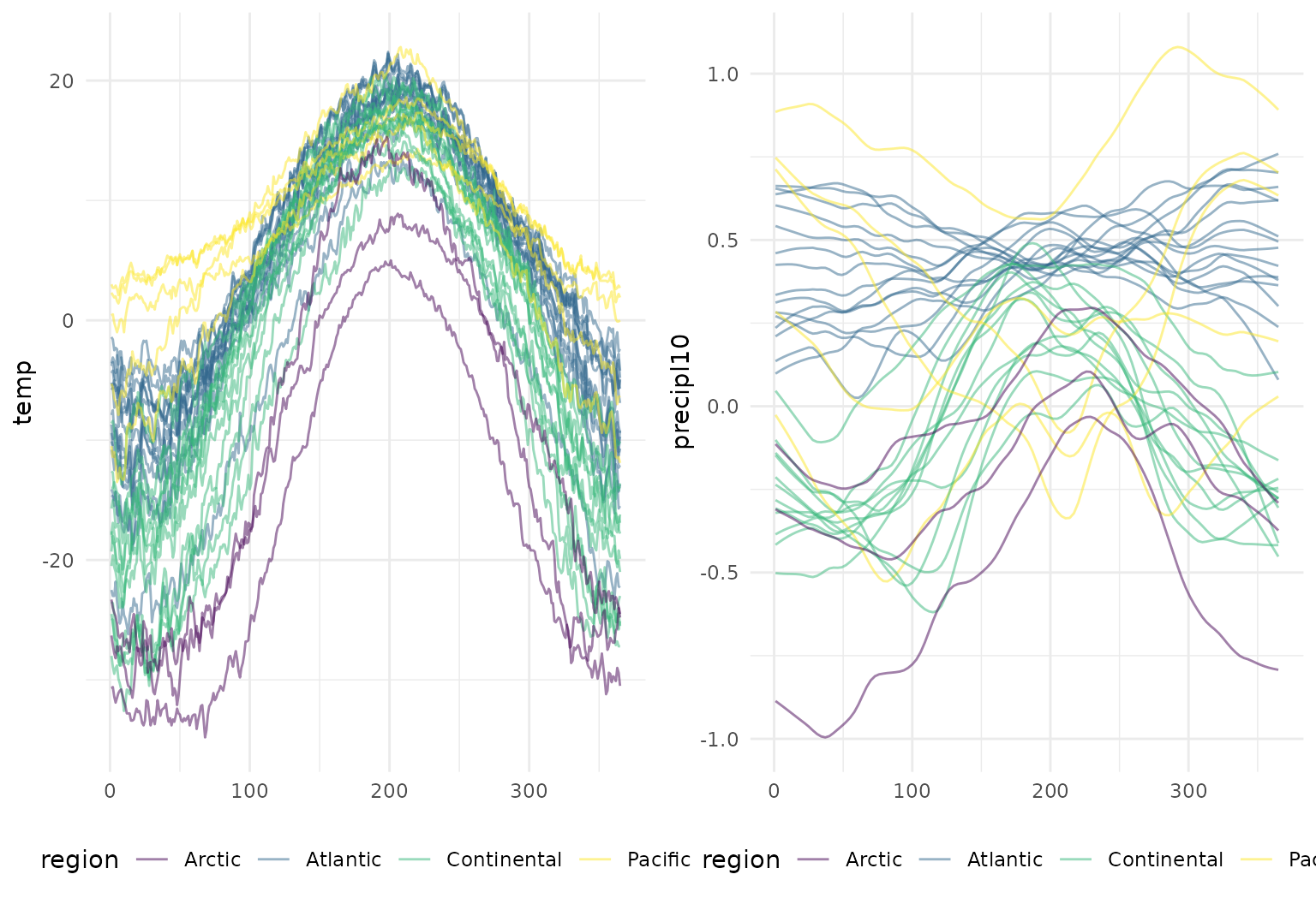

Conversion to `tf` from a data frame

… in “long” format

“Long” format data frames containing functional data include columns containing a subject identifier, the functional argument, and the value each subject’s function takes at each argument. There are also often (but not always) non-functional covariates that are repeated within a subject. For data in this form, we use tf_nest to produce a data frame containing a single row for each subject.

A first example is the sleepstudy data from the lme4 package, which is a nice example from longitudinal data analysis. This includes columns for Subject, Days, and Reaction – which correspond to the subject, argument, and value.

data("sleepstudy", package = "lme4")
sleepstudy <- as_tibble(sleepstudy)

sleepstudy
## # A tibble: 180 × 3
##    Reaction  Days Subject
##       <dbl> <dbl> <fct>  
##  1     250.     0 308    
##  2     259.     1 308    
##  3     251.     2 308    
##  4     321.     3 308    
##  5     357.     4 308    
##  6     415.     5 308    
##  7     382.     6 308    
##  8     290.     7 308    
##  9     431.     8 308    
## 10     466.     9 308    
## # ℹ 170 more rows

We create sleepstudy_tf by nesting Reaction within subjects. The result is a data frame containing a single row for each curve (one per Subject) that holds two columns: the Reaction function and the Subject ID:

sleepstudy_tf <- sleepstudy |>
  tf_nest(Reaction, .id = Subject, .arg = Days)

sleepstudy_tf
## # A tibble: 18 × 2
##    Subject   Reaction
##    <fct>    <tfd_reg>
##  1 308     ▂▂▂▄▅▇▆▃▇█
##  2 309     ▁▁▁▁▁▁▁▁▁▂
##  3 310     ▁▁▂▂▂▁▂▂▂▂
##  4 330     ▄▄▃▃▃▄▃▄▄▅
##  5 331     ▃▃▄▄▄▃▃▅▃▆
##  6 332     ▂▂▃▄▄▄█▅▄▂
##  7 333     ▃▃▃▄▄▅▅▅▅▅
##  8 334     ▃▃▂▂▃▃▄▅▅▆
##  9 335     ▂▃▂▃▂▂▂▂▂▂
## 10 337     ▄▄▃▅▆▆▇▇██
## 11 349     ▂▂▂▂▂▃▃▄▅▅
## 12 350     ▂▂▂▂▃▄▆▅▆▆
## 13 351     ▂▄▃▃▃▄▃▃▄▅
## 14 352     ▁▄▄▅▅▅▅▅▆▆
## 15 369     ▃▃▂▃▄▄▄▅▅▆
## 16 370     ▁▂▂▂▃▅▃▅▆▆
## 17 371     ▃▃▃▃▃▃▂▄▅▆
## 18 372     ▃▃▄▄▃▄▅▅▆▅

We’ll make a quick plot to show the result.

sleepstudy_tf |>
  tf_ggplot(aes(tf = Reaction)) +
  geom_line()

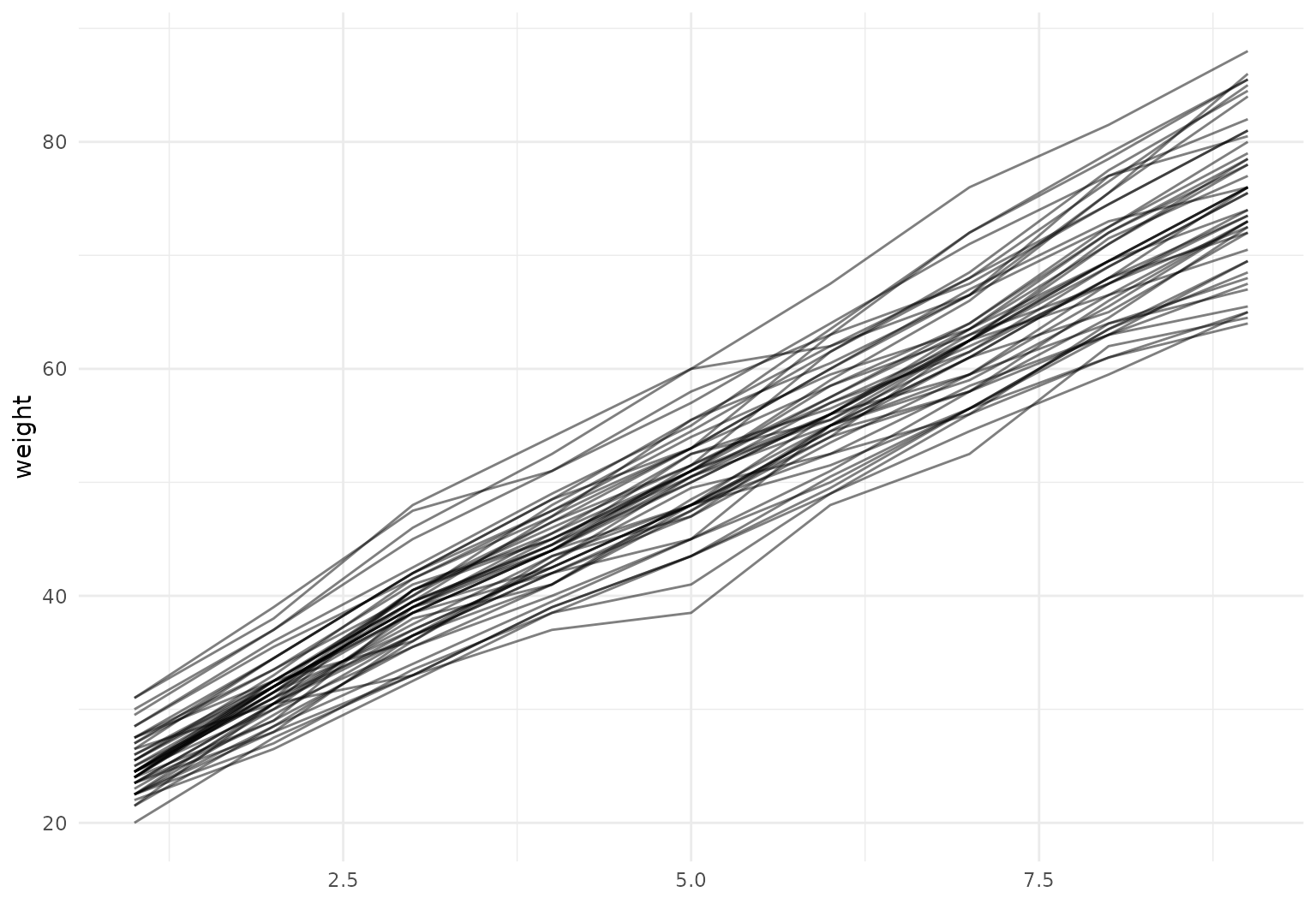
Alternatively, for this simple example that does not contain any additional time-varying or time-constant covariates besides the values that define the functions themselves, we could have simply done:

tibble(
  Subject = unique(sleepstudy$Subject), 
  Reaction = tfd(sleepstudy, id = "Subject", arg = "Days", value = "Reaction")
)
## # A tibble: 18 × 2
##    Subject   Reaction
##    <fct>    <tfd_reg>
##  1 308     ▂▂▂▄▅▇▆▃▇█
##  2 309     ▁▁▁▁▁▁▁▁▁▂
##  3 310     ▁▁▂▂▂▁▂▂▂▂
##  4 330     ▄▄▃▃▃▄▃▄▄▅
##  5 331     ▃▃▄▄▄▃▃▅▃▆
##  6 332     ▂▂▃▄▄▄█▅▄▂
##  7 333     ▃▃▃▄▄▅▅▅▅▅
##  8 334     ▃▃▂▂▃▃▄▅▅▆
##  9 335     ▂▃▂▃▂▂▂▂▂▂
## 10 337     ▄▄▃▅▆▆▇▇██
## 11 349     ▂▂▂▂▂▃▃▄▅▅
## 12 350     ▂▂▂▂▃▄▆▅▆▆
## 13 351     ▂▄▃▃▃▄▃▃▄▅
## 14 352     ▁▄▄▅▅▅▅▅▆▆
## 15 369     ▃▃▂▃▄▄▄▅▅▆
## 16 370     ▁▂▂▂▃▅▃▅▆▆
## 17 371     ▃▃▃▃▃▃▂▄▅▆
## 18 372     ▃▃▄▄▃▄▅▅▆▅

A second example uses the ALA::fev1 dataset. ALA is not on CRAN, so we do not show an install command here. The code below is illustrative only and is not evaluated when the vignette is built.

In this dataset, both height and logFEV1 are observed at multiple ages for each child; that is, there are two functions observed simultaneously, over a shared argument. We can use tf_nest to create a dataframe with a single row for each subject, which includes both non-functional covariates (like age and height at baseline), and functional observations logFEV1 and height.

ALA::fev1 |>
  group_by(id) |>
  mutate(n_obs = n()) |>
  filter(n_obs > 1) |>
  ungroup() |>
  tf_nest(logFEV1, height, .arg = age) |>
  glimpse()

… in “wide” format

In some cases functional data are stored in “wide” format, meaning that there are separate columns for each argument, and values are stored in these columns. In this case, tf_gather can be use to collapse across columns to produce a function for each subject.

The example below again uses the refund::DTI dataset. We use tf_gather to transfer the cca observations from a matrix column (with NAs) into a column of irregularly observed functions (tfd_irreg).

dti_df <- refund::DTI |>
  janitor::clean_names() |>
  select(-starts_with("rcst")) |>
  glimpse()
## Rows: 382
## Columns: 8
## $ id         <dbl> 1001, 1002, 1003, 1004, 1005, 1006, 1007, 1008, 1009, 1010,…
## $ visit      <int> 1, 1, 1, 1, 1, 1, 1, 1, 1, 1, 1, 1, 1, 1, 1, 1, 1, 1, 1, 1,…
## $ visit_time <int> 0, 0, 0, 0, 0, 0, 0, 0, 0, 0, 0, 0, 0, 0, 0, 0, 0, 0, 0, 0,…
## $ nscans     <int> 1, 1, 1, 1, 1, 1, 1, 1, 1, 1, 1, 1, 1, 1, 1, 1, 1, 1, 1, 1,…
## $ case       <dbl> 0, 0, 0, 0, 0, 0, 0, 0, 0, 0, 0, 0, 0, 0, 0, 0, 0, 0, 0, 0,…
## $ sex        <fct> female, female, male, male, male, male, male, male, male, m…
## $ pasat      <int> NA, NA, NA, NA, NA, NA, NA, NA, NA, NA, NA, NA, NA, NA, NA,…
## $ cca        <dbl[,93]> <matrix[26 x 93]>

dti_df |>
  tf_gather(starts_with("cca")) |>
  glimpse()
## creating new <tfd>-column "cca"
## Rows: 382
## Columns: 8
## $ id         <dbl> 1001, 1002, 1003, 1004, 1005, 1006, 1007, 1008, 1009, 1010,…
## $ visit      <int> 1, 1, 1, 1, 1, 1, 1, 1, 1, 1, 1, 1, 1, 1, 1, 1, 1, 1, 1, 1,…
## $ visit_time <int> 0, 0, 0, 0, 0, 0, 0, 0, 0, 0, 0, 0, 0, 0, 0, 0, 0, 0, 0, 0,…
## $ nscans     <int> 1, 1, 1, 1, 1, 1, 1, 1, 1, 1, 1, 1, 1, 1, 1, 1, 1, 1, 1, 1,…
## $ case       <dbl> 0, 0, 0, 0, 0, 0, 0, 0, 0, 0, 0, 0, 0, 0, 0, 0, 0, 0, 0, 0,…
## $ sex        <fct> female, female, male, male, male, male, male, male, male, m…
## $ pasat      <int> NA, NA, NA, NA, NA, NA, NA, NA, NA, NA, NA, NA, NA, NA, NA,…
## $ cca        <tfd_irreg> (1,0.5);(2,0.5);(3,0.5); ..., (1,0.5);(2,0.5);(3,0.5)…

Changing representation with `tf_rebase`

Sometimes you need to make different tf objects compatible – for example, to combine raw observations with a basis representation, or to ensure two functional data vectors are expressed on the same grid or in the same basis. tf_rebase re-expresses one tf object in the representation of another:

# reload the tidyfun version of the DTI data
data(dti_df, package = "tidyfun")

# raw functional data
cca_raw <- dti_df$cca[1:5]
cca_raw
## irregular tfd[5]: [0,1] -> [0.3662524,0.6747586] based on 93 to 93 (mean: 93) evaluations each
## interpolation by tf_approx_linear 
## 1001_1: (0.000,0.49);(0.011,0.52);(0.022,0.54); ...
## 1002_1: (0.000,0.47);(0.011,0.49);(0.022,0.50); ...
## 1003_1: (0.000,0.50);(0.011,0.51);(0.022,0.54); ...
## 1004_1: (0.000,0.40);(0.011,0.42);(0.022,0.44); ...
## 1005_1: (0.000,0.40);(0.011,0.41);(0.022,0.40); ...

# represent in a spline basis
cca_basis <- tfb(dti_df$cca[1:5], k = 25)
## Percentage of input data variability preserved in basis representation
## (per functional observation, approximate):
## Min. 1st Qu.  Median Mean 3rd Qu.  Max.
## 95.60 96.40 96.90 97.12 98.00 98.70
cca_basis
## tfb[5]: [0,1] -> [0.3684063,0.6796841] in basis representation:
##  using  s(arg, bs = "cr", k = 25, sp = -1)  
## 1001_1: ▆██▆▄▃▄▄▄▄▅▅▅▅▅▄▄▂▂▂▃▅▅▆▆▆
## 1002_1: ▅▆▆▄▄▄▄▄▃▄▅▅▄▃▃▃▃▃▃▄▅▆▆▇▆▆
## 1003_1: ▆▇▆▄▃▃▃▃▃▄▃▃▄▄▄▃▃▂▃▃▃▅▆▄▇█
## 1004_1: ▃▅▇▇▆▅▅▄▅▅▅▅▅▅▅▅▄▃▃▃▃▄▅▇▇▆
## 1005_1: ▁▃▅▅▄▂▂▂▃▃▂▃▃▄▃▃▃▃▃▁▁▂▃▅▇▅

# re-express the raw data in the same basis representation
cca_rebased <- tf_rebase(cca_raw, basis_from = cca_basis)
cca_rebased
## tfb[5]: [0,1] -> [0.3684063,0.6796841] in basis representation:
##  using  s(arg, bs = "cr", k = 25, sp = -1)  
## 1001_1: ▆██▆▄▃▄▄▄▄▅▅▅▅▅▄▄▂▂▂▃▅▅▆▆▆
## 1002_1: ▅▆▆▄▄▄▄▄▃▄▅▅▄▃▃▃▃▃▃▄▅▆▆▇▆▆
## 1003_1: ▆▇▆▄▃▃▃▃▃▄▃▃▄▄▄▃▃▂▃▃▃▅▆▄▇█
## 1004_1: ▃▅▇▇▆▅▅▄▅▅▅▅▅▅▅▅▄▃▃▃▃▄▅▇▇▆
## 1005_1: ▁▃▅▅▄▂▂▂▃▃▂▃▃▄▃▃▃▃▃▁▁▂▃▅▇▅

# or convert a spline-based representation to a grid-based one for a specific grid:
tf_rebase(cca_basis, basis_from = cca_raw)
## irregular tfd[5]: [0,1] -> [0.3684063,0.6796841] based on 93 to 93 (mean: 93) evaluations each
## interpolation by tf_approx_linear 
## 1001_1: (0.000,0.49);(0.011,0.52);(0.022,0.54); ...
## 1002_1: (0.000,0.47);(0.011,0.49);(0.022,0.51); ...
## 1003_1: (0.000,0.49);(0.011,0.52);(0.022,0.55); ...
## 1004_1: (0.000,0.41);(0.011,0.42);(0.022,0.44); ...
## 1005_1: (0.000, 0.4);(0.011, 0.4);(0.022, 0.4); ...

This is useful when you want to ensure that operations between tf objects (e.g., addition, comparison) use a common representation, or when you want to convert between tfd and tfb representations while matching a specific basis configuration. It is required for many operations that would otherwise not be well-defined.

Splitting and combining functions

tf_split separates each function into fragments defined on sub-intervals of its domain, and tf_combine joins fragments back together. This is useful for analyzing specific parts of a function separately or for stitching together functional observations from different sources.

# split CCA profiles at their midpoint
cca_halves <- tf_split(dti_df$cca[1:10], splits = 0.5)

# result is a list of tf vectors, one per segment
cca_halves[[1]]
## tfd[10]: [0,0.5] -> [0.3860009,0.6894555] based on 47 evaluations each
## interpolation by tf_approx_linear 
## 1001_1: ▄▅▆▇█▇▇▆▅▃▃▃▃▃▄▄▄▄▄▄▄▄▄▄▄▄
## 1002_1: ▃▄▅▆▆▅▅▃▃▃▄▄▄▄▄▃▃▃▃▃▄▅▅▅▄▄
## 1003_1: ▄▅▇▇▇▆▅▄▃▃▃▃▃▃▃▃▃▃▃▃▃▃▃▃▃▃
## 1004_1: ▁▂▃▄▅▆▆▆▆▅▄▅▅▄▄▄▄▅▄▄▅▅▅▅▅▄
## 1005_1: ▁▁▁▂▃▄▅▅▅▄▂▂▁▂▂▂▂▂▂▂▂▂▂▃▃▃
## 1006_1: ▂▂▃▃▄▅▆▆▆▆▅▄▄▄▄▄▄▄▄▄▅▅▅▅▅▄
##     [....]   (4 not shown)
cca_halves[[2]]
## tfd[10]: [0.5,1] -> [0.3662524,0.7028992] based on 47 evaluations each
## interpolation by tf_approx_linear 
## 1001_1: ▅▅▅▄▄▄▄▄▃▃▂▂▂▂▂▃▄▄▅▅▅▆▆▆▆▆
## 1002_1: ▄▃▃▃▃▃▃▃▃▃▃▃▃▃▄▄▅▅▆▆▆▆▆▆▆▆
## 1003_1: ▄▄▄▄▄▃▃▃▂▂▂▃▃▃▃▃▄▅▅▅▅▃▅▆▇█
## 1004_1: ▄▄▅▅▄▄▄▄▄▃▃▂▂▂▃▃▄▄▄▅▆▆▆▆▆▆
## 1005_1: ▃▄▄▄▃▃▃▂▃▃▃▂▂▂▁▁▁▂▂▃▃▄▆▆▆▅
## 1006_1: ▄▅▅▅▅▄▄▄▄▄▄▄▅▅▅▅▆▆▇▆▇▆▆▅▅▄
##     [....]   (4 not shown)

# recombine
cca_recombined <- tf_combine(cca_halves[[1]], cca_halves[[2]])
## ! removing 10 duplicated points from input data.
cca_recombined 
## tfd[10]: [0,1] -> [0.3662524,0.7028992] based on 93 evaluations each
## interpolation by tf_approx_linear 
## 1: ▄▇▇▆▄▃▃▄▄▄▄▄▄▅▄▄▄▃▂▂▂▄▅▅▆▆
## 2: ▄▆▆▄▃▄▄▄▃▃▄▅▄▃▃▃▃▃▃▄▄▅▆▆▆▆
## 3: ▄▇▆▄▃▃▃▃▃▃▃▃▃▄▄▃▃▂▃▃▃▄▅▄▅█
## 4: ▂▄▆▆▆▅▅▄▄▄▅▅▅▄▅▄▄▃▃▂▃▄▄▆▆▆
## 5: ▁▂▄▅▄▂▂▂▂▃▂▃▃▄▄▃▂▃▃▂▁▁▃▄▆▆
## 6: ▃▄▅▆▆▅▄▄▄▄▅▅▅▅▅▅▄▄▄▅▅▆▆▆▆▄
##     [....]   (4 not shown)

Conversion from `fda` objects

The fda package represents functional data as fd objects (basis function coefficients + basis definition). tf can convert these directly using tfb_spline, which re-expresses the fd basis in tf’s spline framework. This also works for fdSmooth objects returned by fda::smooth.basis.

# create an fd object from the Canadian weather data
weather_basis <- fda::create.fourier.basis(c(0, 365), nbasis = 65)
weather_fd <- fda::smooth.basis(
  argvals = 1:365,
  y = fda::CanadianWeather$dailyAv[, , 1],
  fdParobj = weather_basis
)

# convert fdSmooth to tfb
weather_tf <- tfb_spline(weather_fd)
## Percentage of input data variability preserved in basis representation
## (per functional observation, approximate):
## Min. 1st Qu.  Median Mean 3rd Qu.  Max.
## 100 100 100 100 100 100
weather_tf[1:3]
## tfb[3]: [0,365] -> [-7.867481,19.46969] in basis representation:
##  using  s(arg, bs = "fourier", k = 65, sp = NA, xt = list(period = 365))  
## St. Johns: ▁▁▁▁▂▃▃▃▄▅▅▆▇▇██▇▇▆▅▅▄▃▃▂▂
## Halifax  : ▁▁▁▁▂▃▃▄▅▆▇▇█████▇▇▆▅▅▃▃▂▁
## Sydney   : ▁▁▁▁▂▃▃▄▄▅▆▇▇████▇▆▆▅▄▄▃▂▂

The resulting tfb object can then be used with all tidyfun tools:

tibble(
  place = fda::CanadianWeather$place,
  region = fda::CanadianWeather$region,
  temp = weather_tf
) |>
  tf_ggplot(aes(tf = temp, color = region)) +
  geom_line(alpha = 0.5)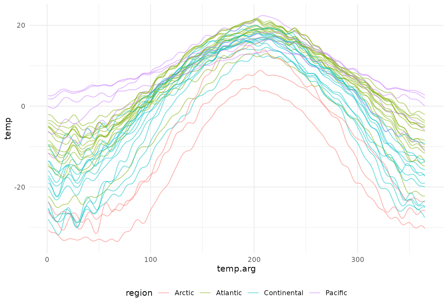

Reversing the conversion

tidyfun includes a wide range of tools for exploratory analysis and visualization, but many analysis approaches require data to be stored in more traditional formats. Several functions are available to aid in this conversion.

Conversion from `tf` to data frames

The functions tf_unnest and tf_spread reverse the operations in tf_nest and tf_gather, respectively – that is, they take a data frame with a functional observation and produce long or wide data frames. We’ll illustrate these with the sleepstudy_tf data set.

First, to produce a long-format data frame, one can use tf_unnest:

sleepstudy_tf |>
  tf_unnest(cols = Reaction) |>
  glimpse()
## Rows: 180
## Columns: 3
## $ Subject        <fct> 308, 308, 308, 308, 308, 308, 308, 308, 308, 308, 309, …
## $ Reaction_arg   <dbl> 0, 1, 2, 3, 4, 5, 6, 7, 8, 9, 0, 1, 2, 3, 4, 5, 6, 7, 8…
## $ Reaction_value <dbl> 249.5600, 258.7047, 250.8006, 321.4398, 356.8519, 414.6…

To produce a wide-format data frame, one can use tf_spread:

sleepstudy_tf |>
  tf_spread() |>
  glimpse()
## Rows: 18
## Columns: 11
## $ Subject    <fct> 308, 309, 310, 330, 331, 332, 333, 334, 335, 337, 349, 350,…
## $ Reaction_0 <dbl> 249.5600, 222.7339, 199.0539, 321.5426, 287.6079, 234.8606,…
## $ Reaction_1 <dbl> 258.7047, 205.2658, 194.3322, 300.4002, 285.0000, 242.8118,…
## $ Reaction_2 <dbl> 250.8006, 202.9778, 234.3200, 283.8565, 301.8206, 272.9613,…
## $ Reaction_3 <dbl> 321.4398, 204.7070, 232.8416, 285.1330, 320.1153, 309.7688,…
## $ Reaction_4 <dbl> 356.8519, 207.7161, 229.3074, 285.7973, 316.2773, 317.4629,…
## $ Reaction_5 <dbl> 414.6901, 215.9618, 220.4579, 297.5855, 293.3187, 309.9976,…
## $ Reaction_6 <dbl> 382.2038, 213.6303, 235.4208, 280.2396, 290.0750, 454.1619,…
## $ Reaction_7 <dbl> 290.1486, 217.7272, 255.7511, 318.2613, 334.8177, 346.8311,…
## $ Reaction_8 <dbl> 430.5853, 224.2957, 261.0125, 305.3495, 293.7469, 330.3003,…
## $ Reaction_9 <dbl> 466.3535, 237.3142, 247.5153, 354.0487, 371.5811, 253.8644,…

Converting back to a matrix or data frame

To convert tf vector to a matrix with each row containing the function evaluations for one function, use as.matrix:

reaction_matrix <- sleepstudy_tf |> pull(Reaction) |> as.matrix() 
 
head(reaction_matrix)
##            0        1        2        3        4        5        6        7
## 308 249.5600 258.7047 250.8006 321.4398 356.8519 414.6901 382.2038 290.1486
## 309 222.7339 205.2658 202.9778 204.7070 207.7161 215.9618 213.6303 217.7272
## 310 199.0539 194.3322 234.3200 232.8416 229.3074 220.4579 235.4208 255.7511
## 330 321.5426 300.4002 283.8565 285.1330 285.7973 297.5855 280.2396 318.2613
## 331 287.6079 285.0000 301.8206 320.1153 316.2773 293.3187 290.0750 334.8177
## 332 234.8606 242.8118 272.9613 309.7688 317.4629 309.9976 454.1619 346.8311
##            8        9
## 308 430.5853 466.3535
## 309 224.2957 237.3142
## 310 261.0125 247.5153
## 330 305.3495 354.0487
## 331 293.7469 371.5811
## 332 330.3003 253.8644

# argument values of input data saved in `arg`-attribute:
attr(reaction_matrix, "arg")
##  [1] 0 1 2 3 4 5 6 7 8 9

To convert a tf vector to a standalone data frame with "id","arg","value"-columns, use as.data.frame() with unnest = TRUE:

sleepstudy_tf |> pull(Reaction) |> 
  as.data.frame(unnest = TRUE) |>
  head()
##        id arg    value
## 308.1 308   0 249.5600
## 308.2 308   1 258.7047
## 308.3 308   2 250.8006
## 308.4 308   3 321.4398
## 308.5 308   4 356.8519
## 308.6 308   5 414.6901

Jeff Goldsmith, Fabian Scheipl

2026-03-19

Conversion from matrices

Conversion to `tf` from a data frame

… in “long” format

… in “wide” format

Changing representation with `tf_rebase`

Splitting and combining functions

Conversion from `fda` objects

Reversing the conversion

Conversion from `tf` to data frames

Converting back to a matrix or data frame

Converting to & from `tf`

Jeff Goldsmith, Fabian Scheipl

2026-03-19

Conversion from matrices

Conversion to tf from a data frame

… in “long” format

… in “wide” format

Changing representation with tf_rebase

Splitting and combining functions

Conversion from fda objects

Reversing the conversion

Conversion from tf to data frames

Converting back to a matrix or data frame

Conversion to `tf` from a data frame

Changing representation with `tf_rebase`

Conversion from `fda` objects

Conversion from `tf` to data frames