Diffusion tensor imaging data

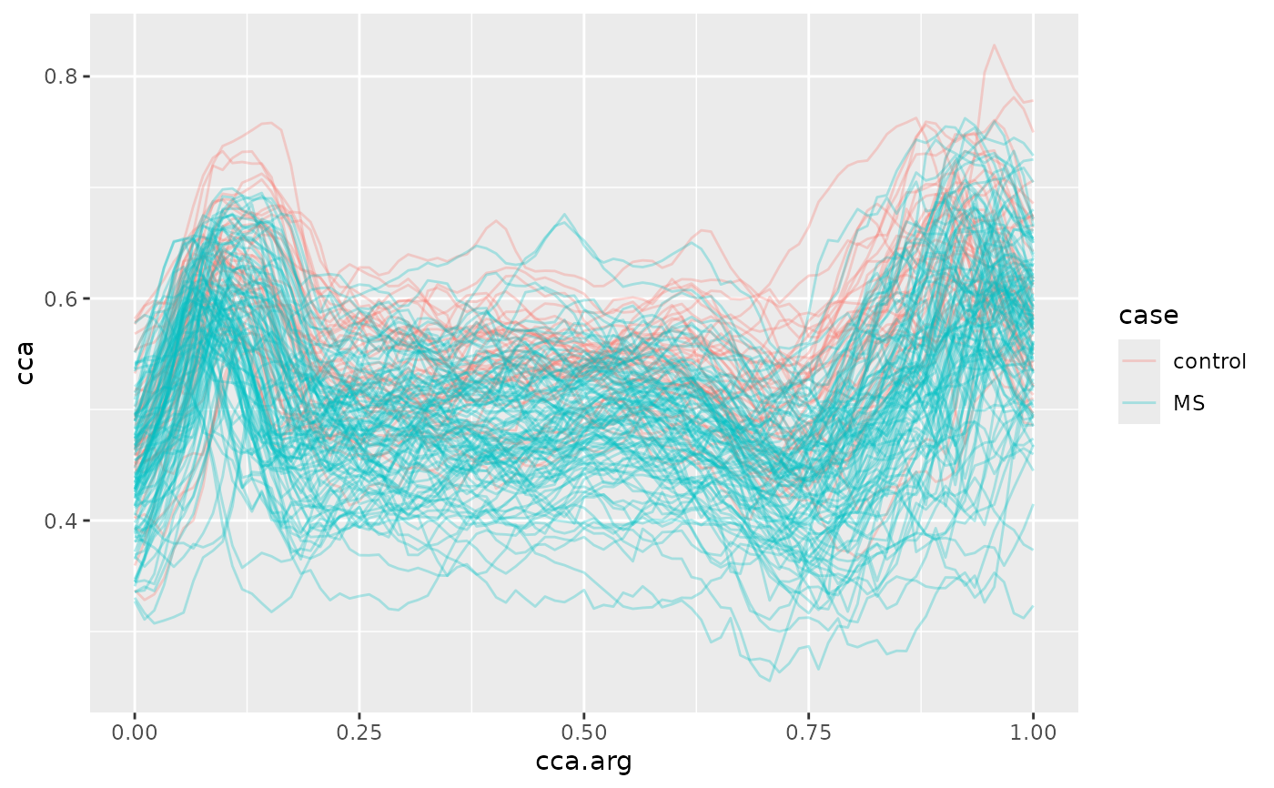
Fractional anisotropy (FA) tract profiles for the corpus callosum (cca) and the right corticospinal tract (rcst) from a diffusion tensor imaging (DTI) study of multiple sclerosis patients and healthy controls.

The original data in refund::DTI include additional variables (pasat, Nscans, visit.time) that were not carried over here.

Usage

dti_df

Format

A tibble with 382 rows and 6 columns:

id

(numeric) Subject identifier.

visit

(integer) Visit number.

sex

(factor) "male" or "female".

case

(factor) "control" or "MS" (multiple sclerosis status).

cca

(tfd_irreg) FA tract profiles for the corpus callosum (up to 93 evaluation points, domain 0–1).

rcst

(tfd_irreg) FA tract profiles for the right corticospinal tract (up to 55 evaluation points, domain 0–1).

Source

Data are from the Johns Hopkins University and the Kennedy-Krieger Institute. Also available in a different format as refund::DTI.

Details

If you use this data as an example in written work, please include the following acknowledgment: "The MRI/DTI data were collected at Johns Hopkins University and the Kennedy-Krieger Institute."

References

Goldsmith, J., Bobb, J., Crainiceanu, C., Caffo, B., and Reich, D. (2011). Penalized Functional Regression. Journal of Computational and Graphical Statistics, 20(4), 830–851. doi:10.1198/jcgs.2010.10007

Goldsmith, J., Crainiceanu, C., Caffo, B., and Reich, D. (2012). Longitudinal Penalized Functional Regression for Cognitive Outcomes on Neuronal Tract Measurements. Journal of the Royal Statistical Society: Series C, 61(3), 453–469. doi:10.1111/j.1467-9876.2011.01031.x

See also

chf_df for another example dataset, vignette("x04_Visualization", package = "tidyfun") for usage examples.

Other tidyfun datasets: chf_df

Examples

dti_df
#> # A tibble: 382 × 6
#>       id visit sex    case                                            cca
#>    <dbl> <int> <fct>  <fct>                                   <tfd_irreg>
#>  1  1001     1 female control (0.000,0.49);(0.011,0.52);(0.022,0.54); ...
#>  2  1002     1 female control (0.000,0.47);(0.011,0.49);(0.022,0.50); ...
#>  3  1003     1 male   control (0.000,0.50);(0.011,0.51);(0.022,0.54); ...
#>  4  1004     1 male   control (0.000,0.40);(0.011,0.42);(0.022,0.44); ...
#>  5  1005     1 male   control (0.000,0.40);(0.011,0.41);(0.022,0.40); ...
#>  6  1006     1 male   control (0.000,0.45);(0.011,0.45);(0.022,0.46); ...
#>  7  1007     1 male   control (0.000,0.55);(0.011,0.56);(0.022,0.56); ...
#>  8  1008     1 male   control (0.000,0.45);(0.011,0.48);(0.022,0.50); ...
#>  9  1009     1 male   control (0.000,0.50);(0.011,0.51);(0.022,0.52); ...
#> 10  1010     1 male   control (0.000,0.46);(0.011,0.47);(0.022,0.48); ...
#> # ℹ 372 more rows
#> # ℹ 1 more variable: rcst <tfd_irreg>

library(ggplot2)
dti_df |>
  dplyr::filter(visit == 1) |>
  tf_ggplot(aes(tf = cca, color = case)) +
  geom_line(alpha = 0.3)