tf Vectors and Operations

This vignette introduces the tf class, as well as the tfd and tfb subclasses, and focuses on vectors of this class. It also illustrates operations for tf vectors.

`tf`-Class: Definition

`tf`-class

tf is a new data type for (vectors of) functional data:

an abstract superclass for functional data in 2 forms:
- as (argument, value)-tuples: subclass tfd, also irregular or sparse
- or in basis representation: subclass tfb represents each observed function as a weighted sum of a fixed dictionary of known “basis functions”.
basically, a list of numeric vectors
(… since lists work well as columns of data frames …)
with additional attributes that define function-like behavior:
- how to evaluate the given “functions” for new arguments
- their domain
- the resolution of the argument values
S3 based

Example Data

First we extract a tf vector from the tidyfun::dti_df dataset containing fractional anisotropy tract profiles for the corpus callosum (cca). When printed, tf vectors show the first few arg and value pairs for each subject.

data("dti_df")

cca <- dti_df$cca
cca
## tfd[382] on (0,1) based on 73 to 93 (mean: 93) evaluations each
## inter-/extrapolation by tf_approx_linear 
## 1001_1: (0.000,0.49);(0.011,0.52);(0.022,0.54); ...
## 1002_1: (0.000,0.47);(0.011,0.49);(0.022,0.50); ...
## 1003_1: (0.000,0.50);(0.011,0.51);(0.022,0.54); ...
## 1004_1: (0.000,0.40);(0.011,0.42);(0.022,0.44); ...
## 1005_1: (0.000,0.40);(0.011,0.41);(0.022,0.40); ...
##     [....]   (377 not shown)

We also extract a simple 5-element vector of functions on a regular grid:

cca_five <- cca[1:5, seq(0, 1, length.out = 93), interpolate = TRUE]
rownames(cca_five) <- LETTERS[1:5]
cca_five <- tfd(cca_five, signif = 2)
cca_five
## tfd[5] on (0,1) based on 93 evaluations each
## interpolation by tf_approx_linear 
## A: (0.000,0.49);(0.011,0.52);(0.022,0.54); ...
## B: (0.000,0.47);(0.011,0.49);(0.022,0.50); ...
## C: (0.000,0.50);(0.011,0.51);(0.022,0.54); ...
## D: (0.000,0.40);(0.011,0.42);(0.022,0.44); ...
## E: (0.000,0.40);(0.011,0.41);(0.022,0.40); ...

For illustration, we plot the vector cca_five below.

plot(cca_five, xlim = c(-0.15, 1), col = pal_5)
text(x = -0.1, y = cca_five[, 0.07], labels = names(cca_five), col = pal_5)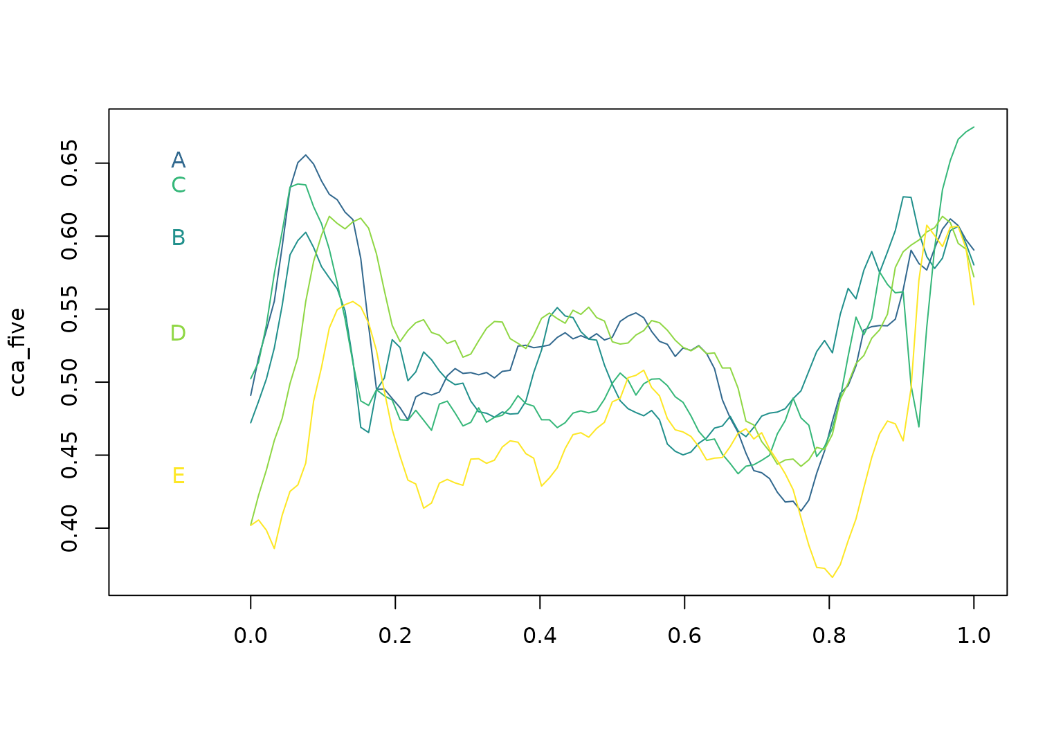

`tf` subclass: `tfd`

tfd objects contain “raw” functional data:

represented as a list of evaluations \(f_i(t)|_{t=t'}\) and corresponding argument vector(s) \(t'\)
has a domain: the range of valid args.

cca_five |>
  tf_evaluations() |>
  str()
## List of 5
##  $ A: num [1:93] 0.491 0.517 0.536 0.555 0.593 ...
##  $ B: num [1:93] 0.472 0.487 0.502 0.523 0.552 ...
##  $ C: num [1:93] 0.502 0.514 0.539 0.574 0.603 ...
##  $ D: num [1:93] 0.402 0.423 0.44 0.46 0.475 ...
##  $ E: num [1:93] 0.402 0.406 0.399 0.386 0.409 ...
cca_five |>
  tf_arg() |>
  str()
##  num [1:93] 0 0.0109 0.0217 0.0326 0.0435 ...
cca_five |> tf_domain()
## [1] 0 1

each tfd-vector contains an evaluator function that defines how to inter-/extrapolate evaluations between args

tf_evaluator(cca_five) |> str()
## function (x, arg, evaluations)
tf_evaluator(cca_five) <- tf_approx_spline

tfd has two subclasses: one for regular data with a common grid and one for irregular or sparse data. The cca data are irregular (values are missing for some subjects at some arguments) but the example below more clearly illustrates support for sparse and irregular data using CD4 cell counts from a longitudinal study.

cd4_vec <- tfd(refund::cd4)

cd4_vec[1:2]
## tfd[2] on (-18,42) based on 3 to 4 (mean: 4) evaluations each
## inter-/extrapolation by tf_approx_linear 
## [1]: (-9,548);(-3,893);( 3,657)
## [2]: (-3,752);( 3,459);( 9,181); ...
cd4_vec[1:2] |>
  tf_arg() |>
  str()
## List of 2
##  $ : num [1:3] -9 -3 3
##  $ : num [1:4] -3 3 9 15
cd4_vec[1:20] |> plot(pch = "x", col = viridis(20))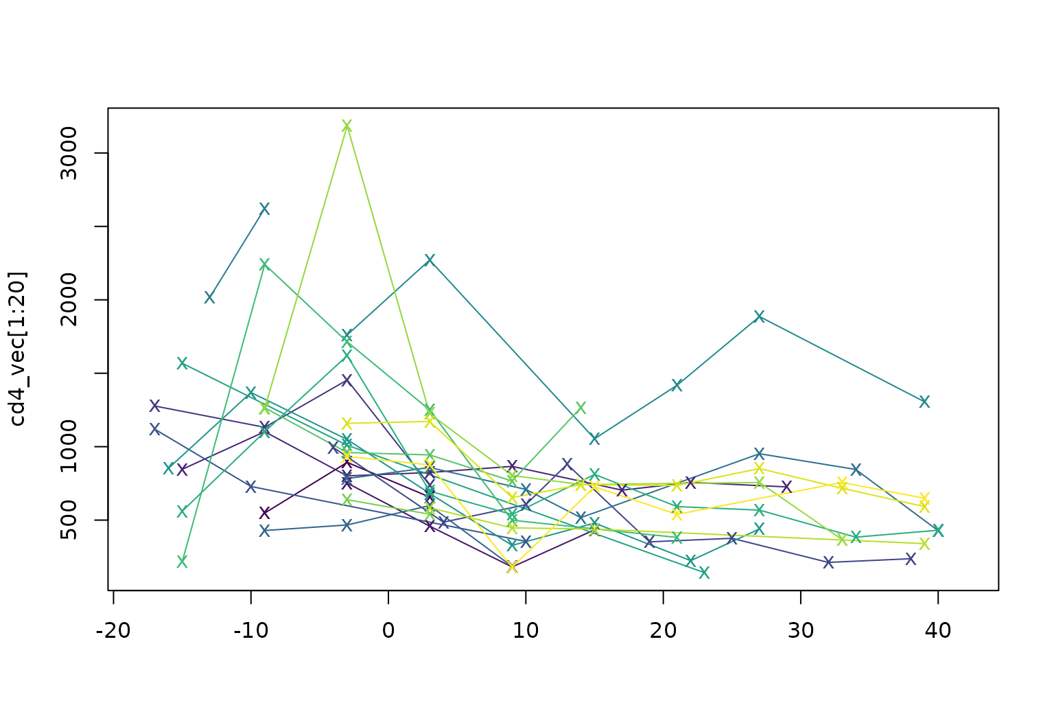

`tf` subclass: `tfb`

Functional data in basis representation:

represented as a list of coefficients and a common basis_matrix of basis function evaluations on a vector of arg-values.
contains a basis function that defines how to evaluate the basis functions for new args and how to differentiate or integrate it.
(internal) flavors:
- tfb_spline: uses mgcv-spline bases
- tfb_fpc: uses functional principal components
significant memory and time savings:

refund::DTI$cca |>
  object.size() |>
  print(units = "Kb")
## 307.7 Kb
cca |>
  object.size() |>
  print(units = "Kb")
## 782.4 Kb
cca |>
  tfb(verbose = FALSE) |>
  object.size() |>
  print(units = "Kb")
## 183.1 Kb

`tfb_spline`: spline basis

default for tfb()
accepts all arguments of mgcv’s s()-syntax: basis type bs, basis dimension k, penalty order m, etc…
also does non-Gaussian fits: family argument
- all exponential families
- but also: \(t\)-distribution, ZI-Poisson, Beta, …

cca_five_b <- cca_five |> tfb()
## Percentage of input data variability preserved in basis representation
## (per functional observation, approximate):
##    Min. 1st Qu.  Median    Mean 3rd Qu.    Max. 
##   95.60   96.40   96.90   97.12   98.00   98.70
cca_five_b[1:2]
## tfb[2] on (0,1) in basis representation:
##  using  s(arg, bs = "cr", k = 25, sp = -1) 
## A: (0.000,0.49);(0.011,0.52);(0.022,0.54); ...
## B: (0.000,0.47);(0.011,0.49);(0.022,0.51); ...
cca_five[1:2] |> tfb(bs = "tp", k = 55)
## Percentage of input data variability preserved in basis representation
## (per functional observation, approximate):
##    Min. 1st Qu.  Median    Mean 3rd Qu.    Max. 
##   99.10   99.22   99.35   99.35   99.47   99.60
## tfb[2] on (0,1) in basis representation:
##  using  s(arg, bs = "tp", k = 55, sp = -1) 
## A: (0.000,0.49);(0.011,0.52);(0.022,0.54); ...
## B: (0.000,0.47);(0.011,0.49);(0.022,0.50); ...

# functions represent ratios in (0,1), so a Beta-distribution is more appropriate:
cca_five[1:2] |>
  tfb(bs = "ps", m = c(2, 1), family = mgcv::betar(link = "cloglog"))
## Percentage of input data variability preserved in basis representation
## (on inverse link-scale, per functional observation, approximate):
##    Min. 1st Qu.  Median    Mean 3rd Qu.    Max. 
##   99.40   99.47   99.55   99.55   99.62   99.70
## tfb[2] on (0,1) in basis representation:
##  using  s(arg, bs = "ps", k = 25, m = c(2, 1), sp = -1) 
## A: (0.000,0.49);(0.011,0.51);(0.022,0.54); ...
## B: (0.000,0.47);(0.011,0.49);(0.022,0.51); ...

Penalization:

Function-specific (default), none, prespecified (sp), or global:

layout(t(1:2))
cca_five |> plot()
cca_five_b |> plot(col = "red")
cca_five |>
  tfb(k = 35, penalized = FALSE) |>
  lines(col = "blue")
## Percentage of input data variability preserved in basis representation
## (per functional observation, approximate):
##    Min. 1st Qu.  Median    Mean 3rd Qu.    Max. 
##    98.5    98.6    98.7    99.0    99.6    99.6
cca_five |>
  tfb(sp = 0.001) |>
  lines(col = "orange")
## Percentage of input data variability preserved in basis representation
## (per functional observation, approximate):
##    Min. 1st Qu.  Median    Mean 3rd Qu.    Max. 
##   72.60   75.90   76.50   76.54   77.20   80.50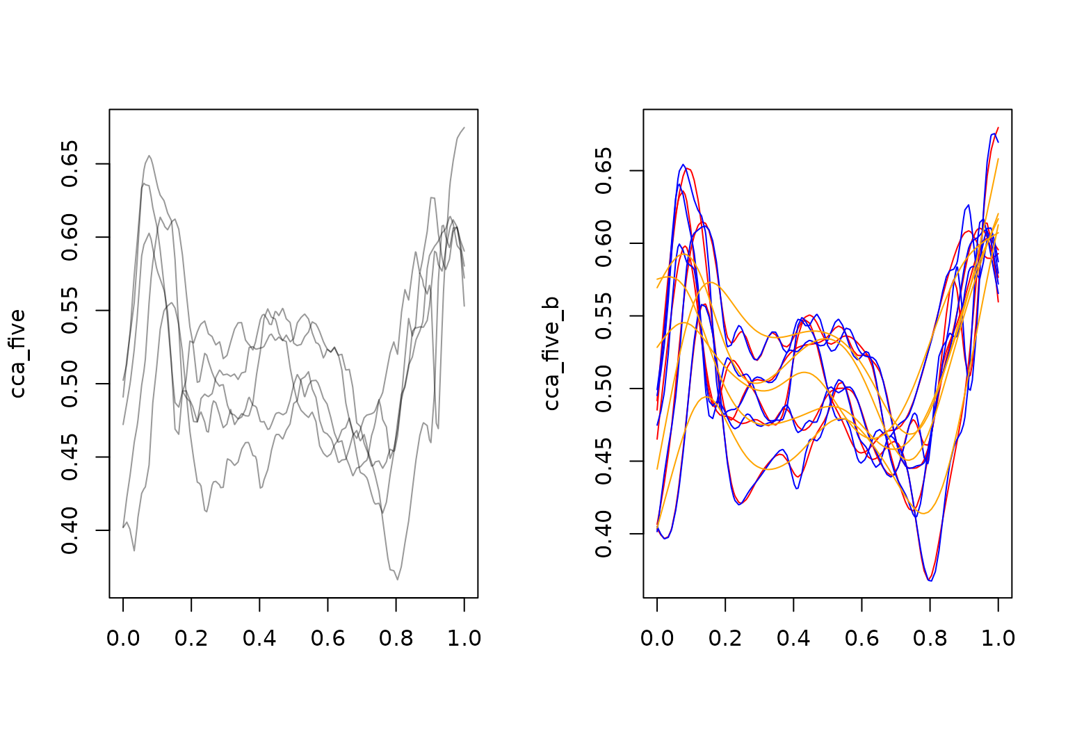

Right plot shows smoothing with function-specific penalization in red, without penalization in blue, and with manually set strong smoothing (sp \(\to 0\)) in orange.

“Global” smoothing:

estimate smoothing parameters for subsample (~10%) of curves
apply geometric mean of estimated smoothing parameters to smooth all curves

Advantages:

(much) faster than optimizing penalization for each curve
should scale well for larg-ish datasets

Disadvantages

no real borrowing of information across curves (very sparse or functional fragment data, e.g.)
still requires more observations than basis functions per curve
subsample could miss small subgroups with different roughness, over-/undersmooth parts of the data, see below.

Dataset with heterogeneous roughness:

layout(t(1:3))
clrs <- scales::alpha(sample(viridis(15)), 0.5)
plot(raw, main = "raw", col = clrs)
plot(tfb(raw, k = 55), main = "separate", col = clrs)
## Percentage of input data variability preserved in basis representation
## (per functional observation, approximate):
##    Min. 1st Qu.  Median    Mean 3rd Qu.    Max. 
##   72.20   88.65   94.80   92.06   96.55   97.70
plot(tfb(raw, k = 55, global = TRUE), main = "global", col = clrs)
## Using global smoothing parameter sp = 3.25e-05, estimated on subsample of curves.
## Percentage of input data variability preserved in basis representation
## (per functional observation, approximate):
##    Min. 1st Qu.  Median    Mean 3rd Qu.    Max. 
##   71.20   80.35   86.40   86.46   95.00   96.90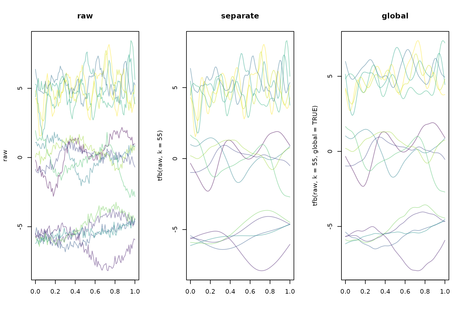

`tfb` FPC-based

uses first few eigenfunctions computed from a simple unregularized (weighted) SVD of the data matrix by default
corresponding FPC basis and mean function saved as tfd-object
observed functions are linear combinations of those.
amount of “smoothing” can be controlled (roughly!) by setting the minimal percentage of variance explained pve

cca_five_fpc <- cca_five |> tfb_fpc(pve = 0.999)
cca_five_fpc
## tfb[5] on (0,1) in basis representation:
##  using  4 FPCs 
## A: (0.000,0.49);(0.011,0.52);(0.022,0.54); ...
## B: (0.000,0.47);(0.011,0.49);(0.022,0.50); ...
## C: (0.000,0.50);(0.011,0.51);(0.022,0.54); ...
## D: (0.000,0.40);(0.011,0.42);(0.022,0.44); ...
## E: (0.000,0.40);(0.011,0.41);(0.022,0.40); ...

cca_five_fpc_lowrank <- cca_five |> tfb_fpc(pve = 0.6)
cca_five_fpc_lowrank
## tfb[5] on (0,1) in basis representation:
##  using  2 FPCs 
## A: (0.000,0.46);(0.011,0.48);(0.022,0.50); ...
## B: (0.000,0.49);(0.011,0.51);(0.022,0.53); ...
## C: (0.000,0.50);(0.011,0.52);(0.022,0.53); ...
## D: (0.000,0.41);(0.011,0.44);(0.022,0.45); ...
## E: (0.000, 0.4);(0.011, 0.4);(0.022, 0.4); ...

layout(t(1:2))
cca_five |> plot()
cca_five_fpc |> plot(col = "red", ylab = "tfb_fpc(cca_five)")
cca_five_fpc_lowrank |> lines(col = "blue", lty = 2)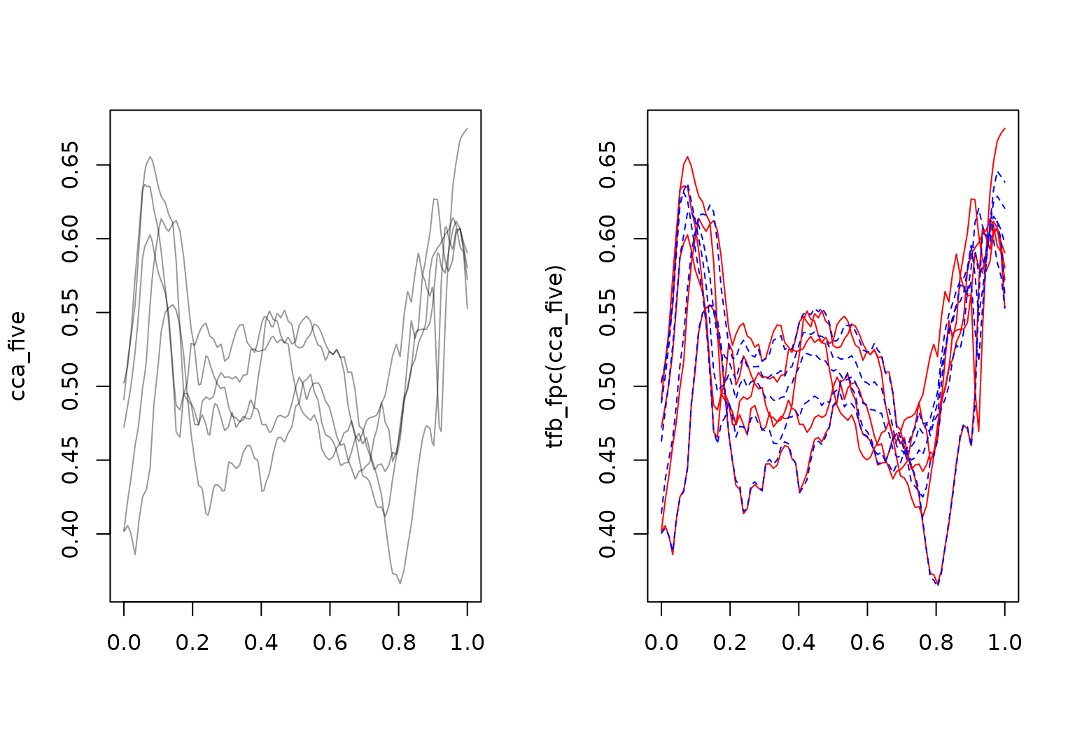

tfb_fpc is currently only implemented for data on identical (but possibly non-equidistant) grids. The {refunder} rfr_fpca-functions provide FPCA methods appropriate for highly irregular and sparse data and regularized/smoothed FPCA.

`tf`-Class: Methods

tidyfun implements almost all types of operations that are available for conventional numerical or logical vectors for tf-vectors as well, so you can:

subset & subassign:

cca_five[1:2]
## tfd[2] on (0,1) based on 93 evaluations each
## interpolation by tf_approx_spline 
## A: (0.000,0.49);(0.011,0.52);(0.022,0.54); ...
## B: (0.000,0.47);(0.011,0.49);(0.022,0.50); ...
cca_five[1:2] <- cca_five[2:1]
cca_five
## tfd[5] on (0,1) based on 93 evaluations each
## interpolation by tf_approx_spline 
## B: (0.000,0.47);(0.011,0.49);(0.022,0.50); ...
## A: (0.000,0.49);(0.011,0.52);(0.022,0.54); ...
## C: (0.000,0.50);(0.011,0.51);(0.022,0.54); ...
## D: (0.000,0.40);(0.011,0.42);(0.022,0.44); ...
## E: (0.000,0.40);(0.011,0.41);(0.022,0.40); ...

compare & compute:

cca_five[1] + cca_five[1] == 2 * cca_five[1]
## [1] TRUE
log(exp(cca_five[2])) == cca_five[2]
## [1] TRUE
(cca_five - (2:-2)) != cca_five
## [1]  TRUE  TRUE FALSE  TRUE  TRUE

summarize across a vector of functions:

Compute functional summaries like mean functions, functional standard deviations or variances or functional data depths over a vector of functional data:

c(mean = mean(cca_five), sd = sd(cca_five))
## tfd[2] on (0,1) based on 93 evaluations each
## interpolation by tf_approx_spline 
## mean: (0.000, 0.45);(0.011, 0.47);(0.022, 0.48); ...
## sd: (0.000,0.049);(0.011,0.052);(0.022,0.062); ...

tf_depth(cca_five) ## Modified Band-2 Depth (à la Sun/Genton/Nychka, 2012), others to come.
##         B         A         C         D         E 
## 0.6108696 0.6467391 0.6597826 0.5728261 0.5097826
median(cca_five) == cca_five[which.max(tf_depth(cca_five))]
##    C 
## TRUE
summary(cca_five)
## tfd[5] on (0,1) based on 93 evaluations each
## interpolation by tf_approx_spline 
## mean: (0.000,  0.45);(0.011,  0.47);(0.022,  0.48); ...
## var: (0.000,0.0024);(0.011,0.0027);(0.022,0.0038); ...
## median: (0.000,  0.50);(0.011,  0.51);(0.022,  0.54); ...
## upper_mid: (0.000,  0.40);(0.011,  0.41);(0.022,  0.40); ...
## lower_mid: (0.000,  0.47);(0.011,  0.49);(0.022,  0.50); ...

summarize each function over its domain:

Compute summaries for each function like its mean or extreme values, quantiles, etc.

tf_fmean(cca_five) # mean of each function's evaluations
##         B         A         C         D         E 
## 0.5202229 0.5266713 0.5090638 0.5308612 0.4661378
tf_fmax(cca_five) # max of each function's evaluations
##         B         A         C         D         E 
## 0.6269639 0.6556130 0.6747586 0.6135842 0.6075271
# 25%-tile of each f(t) for t > .5:
tf_fwise(cca_five, \(x) quantile(x$value[x$arg > 0.5], prob = 0.25)) |> unlist()
##     B.25%     A.25%     C.25%     D.25%     E.25% 
## 0.4747946 0.4675452 0.4650627 0.4770205 0.4462774

tf_fwise can be used to define custom statistics for each function that can depend on both its value and its arg.

In addition, tidyfun provides methods for operations that are specific for functional data:

Methods for “functional” operations

evaluate:

tf-objects have a special [-operator: Its second argument specifies argument values at which to evaluate the functions and has some additional options, so it’s easy to get point values for tf objects, in matrix or data.frame formats:

cca_five[1:2, seq(0, 1, length.out = 3)]
##           0       0.5         1
## B 0.4721627 0.4984125 0.5802742
## A 0.4909345 0.5307563 0.5904773
## attr(,"arg")
## [1] 0.0 0.5 1.0
cca_five["B", seq(0, 0.15, length.out = 3), interpolate = FALSE]
##           0 0.075 0.15
## B 0.4721627    NA   NA
## attr(,"arg")
## [1] 0.000 0.075 0.150
cca_five[1:2, seq(0, 1, length.out = 7), matrix = FALSE] |> str()
## List of 2
##  $ B:'data.frame':   7 obs. of  2 variables:
##   ..$ arg  : num [1:7] 0 0.167 0.333 0.5 0.667 ...
##   ..$ value: num [1:7] 0.472 0.475 0.476 0.498 0.475 ...
##  $ A:'data.frame':   7 obs. of  2 variables:
##   ..$ arg  : num [1:7] 0 0.167 0.333 0.5 0.667 ...
##   ..$ value: num [1:7] 0.491 0.521 0.504 0.531 0.472 ...

(simple, local) smoothing

layout(t(1:3))
cca_five |> plot(alpha = 0.2, ylab = "lowess")
cca_five |>
  tf_smooth("lowess") |>
  lines(col = pal_5)
## using f = 0.15 as smoother span for lowess

cca_five |> plot(alpha = 0.2, ylab = "rolling median (k=5)")
cca_five |>
  tf_smooth("rollmedian", k = 5) |>
  lines(col = pal_5)
## Warning: non-equidistant arg-values in 'cca_five' ignored by rollmedian.
## setting fill = 'extend' for start/end values.

cca_five |> plot(alpha = 0.2, ylab = "Savitzky-Golay (quartic, 11 steps)")
cca_five |>
  tf_smooth("savgol", fl = 11) |>
  lines(col = pal_5)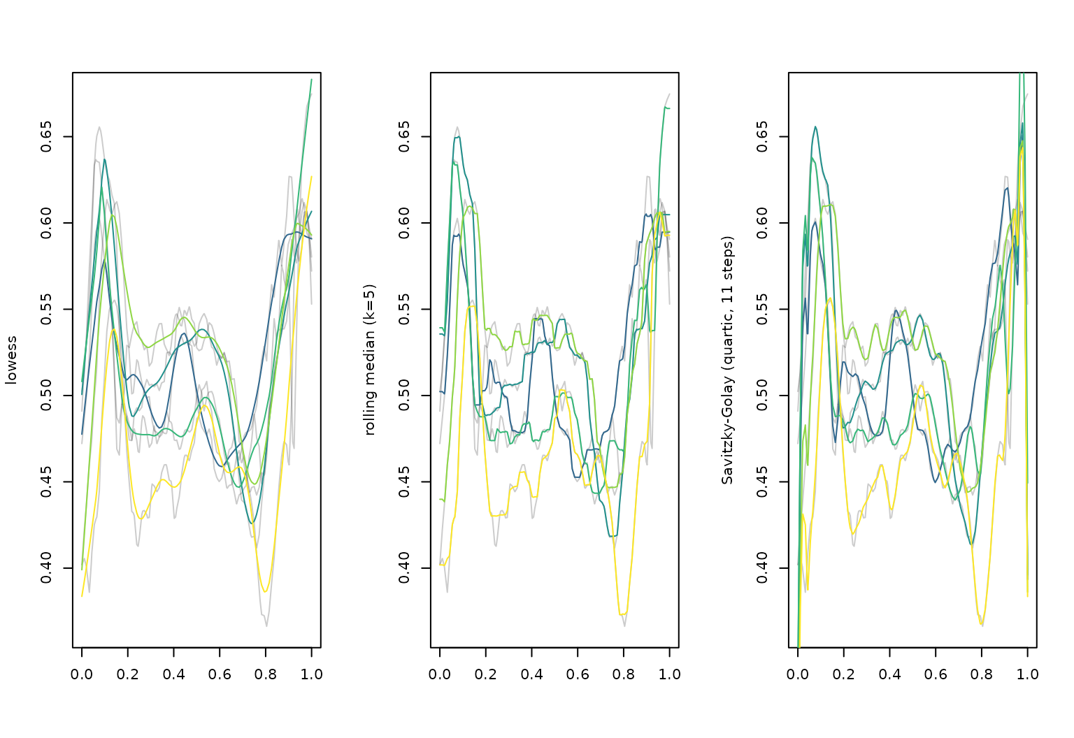
## Warning: non-equidistant arg-values in 'cca_five' ignored by savgol.

differentiate & integrate:

layout(t(1:3))
cca_five |> plot(col = pal_5)
cca_five |>
  tf_smooth() |>
  tf_derive() |>
  plot(col = pal_5, ylab = "tf_derive(tf_smooth(cca_five))")
## using f = 0.15 as smoother span for lowess
cca_five |>
  tf_integrate(definite = FALSE) |>
  plot(col = pal_5)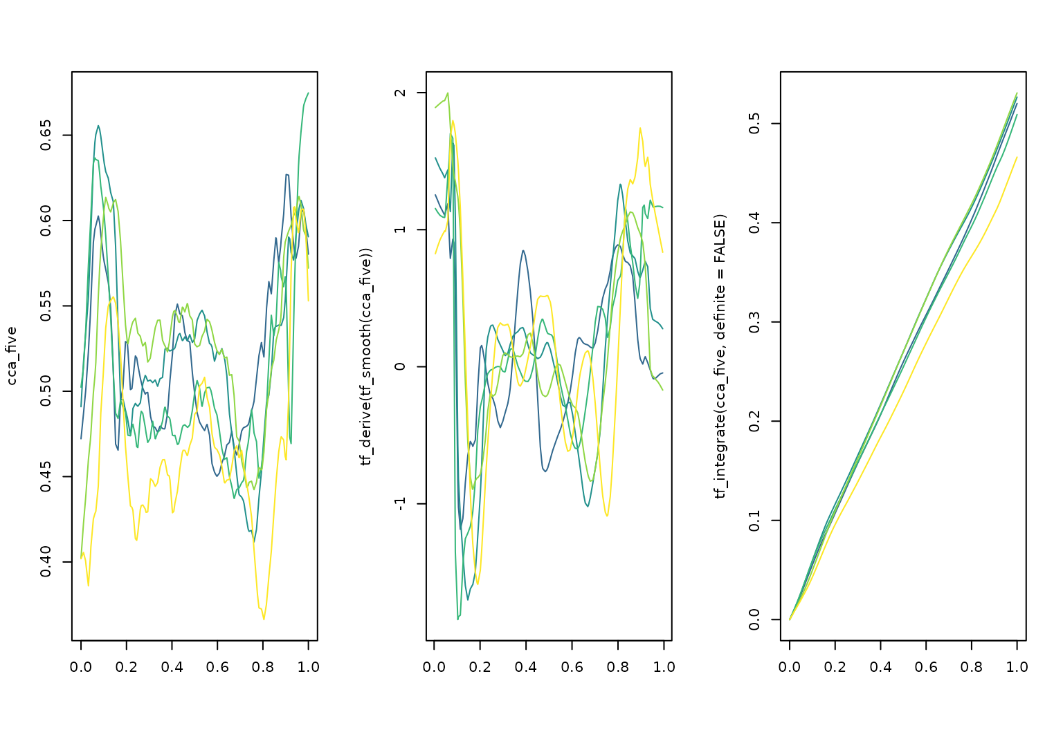

cca_five |> tf_integrate()
##         B         A         C         D         E 
## 0.5202229 0.5266713 0.5090638 0.5308612 0.4661378

query

tidyfun makes it easy to find (ranges of) arguments \(t\) satisfying a condition on value \(f(t)\) (and argument \(t\)):

cca_five |> tf_anywhere(value > 0.65)
##     B     A     C     D     E 
## FALSE  TRUE  TRUE FALSE FALSE
cca_five[1:2] |> tf_where(value > 0.6, "all")
## $B
## [1] 0.07608696 0.89130435 0.90217391 0.91304348 0.92391304 0.96739130 0.97826087
## 
## $A
##  [1] 0.05434783 0.06521739 0.07608696 0.08695652 0.09782609 0.10869565
##  [7] 0.11956522 0.13043478 0.14130435 0.95652174 0.96739130 0.97826087
cca_five[2] |> tf_where(value > 0.6, "range")
##        begin       end
## A 0.05434783 0.9782609
cca_five |> tf_where(value > 0.6 & arg > 0.5, "first")
##         B         A         C         D         E 
## 0.8913043 0.9565217 0.9565217 0.9347826 0.9347826

zoom & query

cca_five |> plot(xlim = c(-0.15, 1), col = pal_5, lwd = 2)
text(x = -0.1, y = cca_five[, 0.07], labels = names(cca_five), col = pal_5, cex = 1.5)
median(cca_five) |> lines(col = pal_5[3], lwd = 4)

# where are the first maxima of these functions?
cca_five |> tf_where(value == max(value), "first")
##          B          A          C          D          E 
## 0.90217391 0.07608696 1.00000000 0.10869565 0.93478261

# where are the first maxima of the later part (t > .5) of these functions?
cca_five[c("A", "D")] |>
  tf_zoom(0.5, 1) |>
  tf_where(value == max(value), "first")
##         A         D 
## 0.9673913 0.9565217

# which f_i(t) are below the functional median anywhere for 0.2 < t < 0.6?
# (t() needed here so we're comparing column vectors to column vectors...)
cca_five |>
  tf_zoom(0.2, 0.6) |>
  tf_anywhere(value <= t(median(cca_five)[, arg]))
##     B     A     C     D     E 
##  TRUE FALSE  TRUE FALSE  TRUE

Jeff Goldsmith, Fabian Scheipl

2024-02-23

`tf`-Class: Definition

`tf`-class

Example Data

`tf` subclass: `tfd`

`tf` subclass: `tfb`

`tfb_spline`: spline basis

Penalization:

`tfb` FPC-based

`tf`-Class: Methods

subset & subassign:

compare & compute:

summarize across a vector of functions:

summarize each function over its domain:

Methods for “functional” operations

evaluate:

(simple, local) smoothing

differentiate & integrate:

query

zoom & query

tf Vectors and Operations

Jeff Goldsmith, Fabian Scheipl

2024-02-23

tf-Class: Definition

tf-class

Example Data

tf subclass: tfd

tf subclass: tfb

tfb_spline: spline basis

Penalization:

tfb FPC-based

tf-Class: Methods

subset & subassign:

compare & compute:

summarize across a vector of functions:

summarize each function over its domain:

Methods for “functional” operations

evaluate:

(simple, local) smoothing

differentiate & integrate:

query

zoom & query

`tf`-Class: Definition

`tf`-class

`tf` subclass: `tfd`

`tf` subclass: `tfb`

`tfb_spline`: spline basis

`tfb` FPC-based

`tf`-Class: Methods