Plot vector-valued functional data

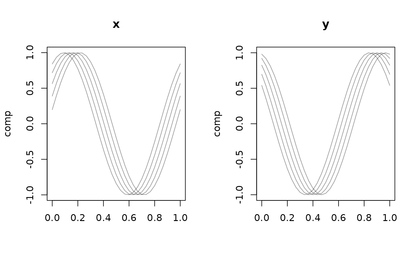
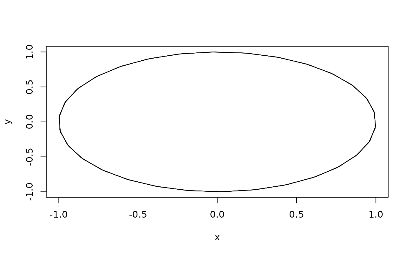
Two simple display modes for tf_mv objects: "facet" draws one panel per output dimension (delegating to the univariate plot.tf()); "trajectory" (only for d == 2) draws the curves in the plane, i.e. \(y(t)\) against \(x(t)\) – the natural view for movement data.

Usage

# S3 method for class 'tf_mv'
plot(x, y, ..., type = NULL)

# S3 method for class 'tf_mv'
lines(x, ..., type = NULL)

# S3 method for class 'tf_mv'
points(x, ..., type = NULL)

Arguments

x

a tf_mv object.

y

ignored.

...

passed to the underlying plotting calls. Per-curve graphical parameters (col, lty, lwd, ...) are recycled across curves.

type

"trajectory" or "facet". Defaults to "trajectory" for two-component (d == 2) objects and to "facet" otherwise.

Value

x, invisibly.

Details

In "trajectory" mode the two components must be paired at common argument values to form \((x(t), y(t))\) points. When the components are sampled on different (or per-curve irregular) grids they are therefore evaluated on the union of their argument grids with interpolate = TRUE (values outside a component's observed range become NA and are skipped). For components that already share a grid this is a no-op.

See also

Other tf_mv-class: tf_arclength(), tf_geom, tf_mv_methods, tfb_mfpc(), tfb_mv(), tfd_mv()

Examples

arg <- seq(0, 1, length.out = 31)
xf <- tfd(t(sapply(1:5, function(i) sin(2 * pi * arg + i / 5))), arg = arg)
yf <- tfd(t(sapply(1:5, function(i) cos(2 * pi * arg + i / 5))), arg = arg)
mv <- tfd_mv(list(x = xf, y = yf))
plot(mv, type = "trajectory")

plot(mv, type = "facet")