Multivariate functional principal component analysis (f: R -> R^d)

tfb_mfpc() computes a multivariate functional principal component analysis (MFPCA) of vector-valued functional data in the sense of Happ & Greven (2018): a single set of scalar scores per curve, shared across all d components, together with vector-valued eigenfunctions $\Psi_m: \mathcal{T} \to \mathbb{R}^d$, so that $f_i(t) \approx \mu(t) + \sum_m s_{im}\,\Psi_m(t)$.

Usage

tfb_mfpc(data, ...)

# S3 method for class 'tf_mv'
tfb_mfpc(
  data,
  weights = c("inverse_variance", "snr", "equal"),
  pve = 0.995,
  npc = NULL,
  uni_pve = 0.995,
  method = fpc_wsvd,
  ...
)

# S3 method for class 'list'
tfb_mfpc(data, arg = NULL, domain = NULL, ...)

# Default S3 method
tfb_mfpc(data, arg = NULL, domain = NULL, ...)

is_tfb_mfpc(x)

tf_mfpc_scores(x)

tf_mfpc_efunctions(x)

Arguments

data: a tfd_mv() / tfb_mv object, a (named) list of univariate tf vectors, or anything tfd_mv() accepts.
...: further arguments forwarded to the univariate method. As in tfb_mv(), a ... argument given as a list named by the component names is distributed per component.
weights: component weighting scheme for the joint analysis. Either a string – "inverse_variance" (default; $w_j = 1 / \sum_l \lambda^{(j)}_l$, so each component contributes equal total variance), "snr" (signal-to-noise: retained variance over the discarded-variance tail of the univariate fit), or "equal" ($w_j = 1$) – or a numeric vector of d non-negative weights. Weights are rescaled to sum to d (so "equal" gives all-ones).
pve: proportion of variance explained used to truncate the multivariate components (default 0.995). Ignored if npc is given.
npc: number of multivariate FPCs to retain (overrides pve).
uni_pve: proportion of variance explained for the univariate FPCA of each component (default 0.995); forwarded as pve to the univariate method.
method: univariate FPCA method, see tfb_fpc(). Defaults to fpc_wsvd().
arg: evaluation grid for raw (list/matrix/array) inputs, forwarded to tfd_mv().
domain: range of arg, forwarded to tfd_mv().
x: a tfb_mv object, ideally one returned by tfb_mfpc().

Value

a tfb_mv object whose d components are tfb_fpc() objects with shared per-curve scores; is_tfb_mfpc() is TRUE for it. Use tf_mfpc_scores() and tf_mfpc_efunctions() to extract the shared scores and the multivariate eigenfunctions.

is_tfb_mfpc(): a logical flag.

tf_mfpc_scores(): an n x M matrix of shared multivariate FPC scores (rows = curves, columns = components).

tf_mfpc_efunctions(): a tfd_mv of length M holding the multivariate eigenfunctions $\Psi_m$ (one "curve" per component).

Details

This is qualitatively different from tfb_mv(data, basis = "fpc"), which fits an independent FPCA per component (separate eigenfunctions and separate scores) and so cannot capture joint variation across dimensions.

The estimator first runs the univariate FPCA (see tfb_fpc() / fpc_wsvd()) on each component to obtain univariate scores $\xi^{(j)}$ and eigenfunctions $\phi^{(j)}$, then eigendecomposes the joint covariance of the (weighted) stacked scores. With component weights $w_j > 0$ the shared scores and multivariate eigenfunctions are $$s_{im} = \sum_j \sqrt{w_j} \sum_l [c_m]^{(j)}_l \xi^{(j)}_{il}, \qquad \Psi_m^{(j)} = \frac{1}{\sqrt{w_j}} \sum_l [c_m]^{(j)}_l \phi^{(j)}_l,$$ where $c_m$ are the eigenvectors of the weighted joint score covariance.

The returned object is a tfb_mv() whose components are tfb_fpc() objects sharing identical per-curve scores; cast it back to evaluations with as.tfd_mv() / vec_cast(), and project new tfd_mv data onto the fitted basis with tf_rebase(). Like the univariate FPCA, the estimator targets data observed on a common grid per component; re-scoring new data evaluates it on each component's estimation grid, so new curves must be observable there.

References

Happ, Clara, Greven, Sonja (2018). “Multivariate functional principal component analysis for data observed on different (dimensional) domains.” Journal of the American Statistical Association, 113(522), 649–659.

Examples

set.seed(1)
g <- tfd_mv(list(hip = tf_rgp(20), knee = tf_rgp(20)))
m <- tfb_mfpc(g, pve = 0.99)
m
#> tfb_mv<d=2>[20] (hip, knee): [0, 1] -> [-2.804624, 1.972252] x [-2.461474, 3.231401]
#> components in basis representation: 8 MFPCs
#> [1]: ▆▆▆▆▆▆▆▆▆▆▆▅▅▅▅▅▅▅▅▅▅▆▆▆▆▆ | ▄▄▄▄▄▄▅▅▅▅▆▆▆▆▆▆▆▅▅▄▄▃▂▂▂▁
#> [2]: ▇▇▇▇▆▆▆▆▆▅▅▅▅▅▅▅▆▆▆▅▅▅▅▅▅▅ | ▃▃▃▃▄▄▄▅▅▅▅▅▅▅▅▄▄▄▃▃▃▃▂▂▂▃
#> [3]: ▆▆▆▆▆▆▆▅▅▄▄▃▃▂▂▂▁▁▁▁▁▁▁▂▂▃ | ▂▁▁▁▂▂▂▂▃▃▃▂▂▂▂▂▁▁▁▁▁▁▁▁▁▂
#> [4]: ▄▄▅▅▆▇▇██████▇▇▆▅▅▅▅▅▅▅▆▆▇ | ▇▇▇▇▆▆▅▅▄▃▃▃▃▃▃▃▃▄▄▅▅▆▆▆▆▆
#> [5]: ▆▆▅▅▄▄▃▃▂▂▂▂▂▂▂▃▃▄▄▄▅▅▅▅▅▅ | ▅▅▅▅▄▄▄▄▄▃▃▃▃▃▃▃▃▄▄▄▄▅▅▅▅▆
#> [6]: ▅▅▅▅▅▅▅▅▅▅▅▅▅▅▅▅▆▆▇▇██████ | ▇▇▇███████▇▇▆▆▅▅▅▄▄▄▄▄▄▄▃▃
#> 
#>     [....]   (14 not shown)
dim(tf_mfpc_scores(m))
#> [1] 20  8
tf_mfpc_efunctions(m)
#> tfd_mv<d=2>[8] (hip, knee): [0, 1] -> [-1.658433, 1.351106] x [-1.564996, 1.729235]
#> components based on 51 evaluations each, interpolation by tf_approx_linear
#> [1]: ▄▄▄▄▃▃▃▃▃▃▂▂▂▂▂▂▂▂▁▁▁▁▁▁▂▂ | ▃▃▃▃▂▂▂▂▁▁▂▂▂▂▂▂▂▂▂▂▃▃▃▃▄▄
#> [2]: ▇▇▇▇▇▆▆▆▆▆▅▅▅▅▄▄▄▃▃▂▂▂▁▁▂▂ | ▆▇▇▇▇▆▆▆▆▆▆▆▆▆▆▅▅▄▄▃▂▁▁▁▁▁
#> [3]: ▂▂▂▂▂▂▂▂▂▂▂▂▂▂▂▂▂▃▃▃▃▃▃▃▃▃ | ▇▇██▇▇▇▇▆▆▆▆▆▆▆▆▆▆▆▆▆▆▆▆▆▆
#> [4]: ▂▂▂▃▄▄▅▆▆▆▆▆▆▆▆▅▅▄▄▄▄▄▅▅▅▅ | █████▇▆▅▄▂▂▁▁▁▁▁▁▂▂▃▃▄▅▅▆▆
#> [5]: ▃▃▃▄▄▅▅▆▆▇▇▇▇▇▇▆▆▅▄▃▂▁▁▁▁▁ | ▄▄▄▃▃▃▃▃▃▃▄▄▄▅▅▆▆▇▇▇▇▇▇▇▇▆
#> [6]: ████▇▇▇▆▆▅▄▄▃▃▂▂▁▁▂▂▃▄▅▆▆▇ | ▄▄▄▄▄▅▅▅▅▅▄▄▃▃▃▃▃▄▅▅▆▇████
#> 
#>     [....]   (2 not shown)
# reconstruct and project new data:
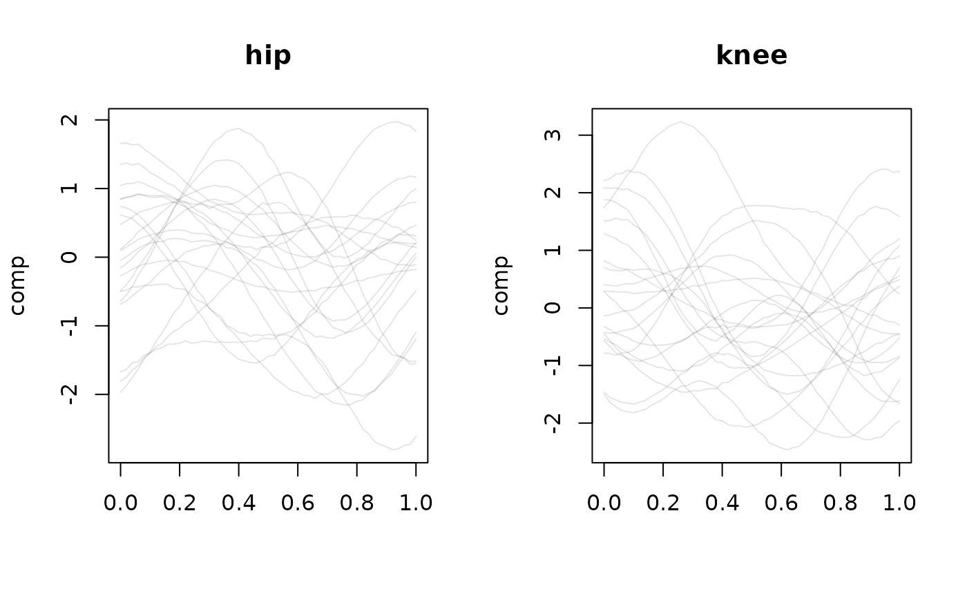
plot(as.tfd_mv(m), type = "facet")

g_new <- tfd_mv(list(hip = tf_rgp(3), knee = tf_rgp(3)))
tf_rebase(g_new, m)
#> tfb_mv<d=2>[3] (hip, knee): [0, 1] -> [-2.211037, 1.183598] x [-1.334569, 1.052306]
#> components in basis representation: 8 MFPCs
#> [1]: ▅▅▅▅▄▄▄▄▄▄▄▄▅▅▅▆▆▆▅▅▅▄▄▃▃▃ | █▇▆▅▃▂▁▁▁▁▂▃▃▄▅▆▆▆▆▆▆▆▅▆▆▆
#> [2]: ▄▄▅▅▅▅▆▆▆▇▇▇▇▇▇▆▆▅▄▃▂▁▁▁▁▁ | ▆▆▆▆▆▆▆▆▆▅▅▄▄▄▃▃▃▃▃▃▄▄▅▆▆▇
#> [3]: █████▇▇▇▇▇▇▇▇▇▇▇▇▇▇▆▆▆▅▅▅▅ | ▇▇▇████████▇▇▆▆▆▅▅▅▅▆▆▇▇▇█
#>

Multivariate functional principal component analysis (`f: R -> R^d`)