Study B: Penalization

Registration Benchmark v2

Setup

library(ggplot2)
library(data.table)
library(patchwork)

base_dir <- here::here()
source(file.path(base_dir, "sim-analyze.R"))

mcols <- method_colors()
mlabs <- method_labels()
dlabs <- dgp_short_labels()

dt <- load_study_b()

study_b_keys <- c("method", "dgp", "noise_sd", "severity")

best <- aggregate_metric(
  dt = dt,
  metric = "warp_mise",
  by = c(study_b_keys, "lambda"),
  stat = "median",
  value_name = "mise"
)
baseline <- best[lambda == 0, .(method, dgp, noise_sd, severity, base = mise)]
optimal <- find_optimal_by_metric(
  dt = dt,
  metric = "warp_mise",
  by = study_b_keys,
  option_col = "lambda",
  stat = "median",
  value_name = "mise"
)
warp_ratio_all <- ratio_to_baseline(
  dt = dt,
  metric = "warp_mise",
  by = c(study_b_keys, "lambda"),
  baseline_col = "lambda",
  baseline_level = 0,
  stat = "median",
  value_name = "mise",
  baseline_name = "base_mise",
  ratio_name = "ratio",
  keep_baseline = TRUE
)
merged <- merge(
  optimal,
  warp_ratio_all[, .(method, dgp, noise_sd, severity, lambda, base_mise, ratio)],
  by = c("method", "dgp", "noise_sd", "severity", "lambda")
)

ae_best <- aggregate_metric(
  dt = dt,
  metric = "alignment_error",
  by = c(study_b_keys, "lambda"),
  stat = "median",
  value_name = "ae"
)
ae_baseline <- ae_best[lambda == 0, .(method, dgp, noise_sd, severity, base = ae)]
ae_optimal <- find_optimal_by_metric(
  dt = dt,
  metric = "alignment_error",
  by = study_b_keys,
  option_col = "lambda",
  stat = "median",
  value_name = "ae"
)
ae_ratio_all <- ratio_to_baseline(
  dt = dt,
  metric = "alignment_error",
  by = c(study_b_keys, "lambda"),
  baseline_col = "lambda",
  baseline_level = 0,
  stat = "median",
  value_name = "ae",
  baseline_name = "base_ae",
  ratio_name = "ratio",
  keep_baseline = TRUE
)
ae_merged <- merge(
  ae_optimal,
  ae_ratio_all[, .(method, dgp, noise_sd, severity, lambda, base_ae, ratio)],
  by = c("method", "dgp", "noise_sd", "severity", "lambda")
)
lambda_comp <- compare_optima(
  opt_a = optimal,
  opt_b = ae_optimal,
  key_cols = study_b_keys,
  value_cols = c("lambda", "lambda"),
  value_names = c("mise_lambda", "ae_lambda")
)

Study B tests whether regularization (lambda > 0) can rescue registration methods in regimes where they struggle. Design: 4 DGPs \(\times\) 8 lambdas \(\times\) 3 methods (SRVF, CC default, CC crit1) \(\times\) 3 noise \(\times\) 2 severity \(\times\) 33 reps = 19,008 runs.

Lambda grid calibrated by pilot (job 5131464): c(0, 1e-4, 1e-3, 0.01, 0.05, 0.1, 1, 10).

cat(sprintf("- Rows: %d | Failures: %d (%.1f%%)\n",
  nrow(dt), sum(dt$failure), 100 * mean(dt$failure)))

• Rows: 19008 | Failures: 0 (0.0%)

cat(sprintf("- DGPs: %s\n", paste(levels(dt$dgp), collapse = ", ")))

• DGPs: D01, D02, D09, D12

cat(sprintf("- Methods: %s\n", paste(levels(dt$method), collapse = ", ")))

• Methods: srvf, cc_default, cc_crit1

cat(sprintf("- Lambdas: %s\n", paste(sort(unique(dt$lambda)), collapse = ", ")))

• Lambdas: 0, 1e-04, 0.001, 0.01, 0.05, 0.1, 1, 10

cat(sprintf("- Noise: %s\n", paste(levels(dt$noise_sd), collapse = ", ")))

• Noise: 0, 0.1, 0.3

Failure rate by lambda

Conditional-on-success MISE comparisons can be biased if failure rates vary by lambda. The table below checks this.

fail_by_lambda <- dt[,
  .(n_total = .N,
    n_fail = sum(failure),
    rate_pct = sprintf("%.1f", 100 * mean(failure))),
  by = .(method, lambda)
]
fail_wide <- dcast(fail_by_lambda,
  method ~ lambda,
  value.var = "rate_pct")
knitr::kable(fail_wide,
  caption = "Failure rate (%) by method and lambda, pooling across DGPs, noise, severity, and reps.")

Failure rate (%) by method and lambda, pooling across DGPs, noise, severity, and reps.

method	0	1e-04	0.001	0.01	0.05	0.1	1	10
srvf	0.0	0.0	0.0	0.0	0.0	0.0	0.0	0.0
cc_default	0.0	0.0	0.0	0.0	0.0	0.0	0.0	0.0
cc_crit1	0.0	0.0	0.0	0.0	0.0	0.0	0.0	0.0

1 MISE vs Lambda Curves

The core question: does the MISE-vs-lambda curve show a U-shape (optimal lambda > 0)?

agg <- dt[failure == FALSE,
  .(mise = median(warp_mise, na.rm = TRUE),
    q25 = quantile(warp_mise, 0.25, na.rm = TRUE),
    q75 = quantile(warp_mise, 0.75, na.rm = TRUE)),
  by = .(method, dgp, noise_sd, severity, lambda)
]

# Baseline (lambda = 0) for reference lines
baseline <- agg[lambda == 0, .(method, dgp, noise_sd, severity, base = mise)]

ggplot(agg[severity == "1"],
  aes(x = lambda + 1e-5, y = mise, color = method)) +
  geom_line(linewidth = 0.6) +
  geom_point(size = 1.5) +
  geom_errorbar(aes(ymin = q25, ymax = q75), width = 0.15, alpha = 0.4) +
  geom_hline(data = baseline[severity == "1"],
    aes(yintercept = base, color = method),
    linetype = "dashed", alpha = 0.5) +
  facet_grid(dgp ~ noise_sd,
    scales = "free_y",
    labeller = labeller(
      noise_sd = function(x) paste0("noise = ", x),
      dgp = dlabs)) +
  scale_x_log10(
    breaks = c(1e-5, 1e-4, 1e-3, 0.01, 0.05, 0.1, 1, 10),
    labels = c("0", "1e-4", "1e-3", "0.01", "0.05", "0.1", "1", "10")) +
  scale_color_manual(values = mcols, labels = mlabs) +
  scale_y_log10() +
  labs(x = expression(lambda ~ "(log scale)"),
    y = "Warp MISE (median, log scale)",
    color = "Method") +
  theme_benchmark() +
  theme(legend.position = "bottom")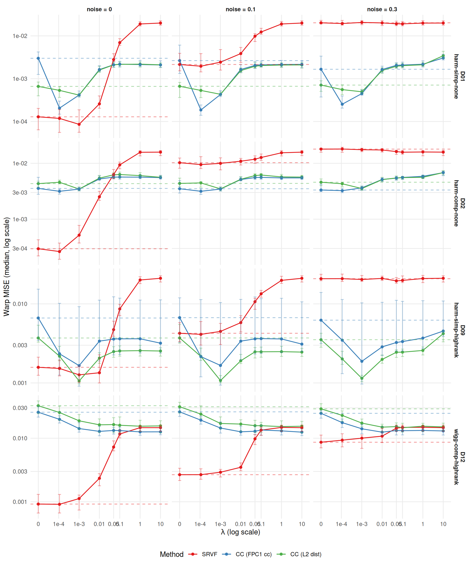

Median warp MISE vs lambda for each method, faceted by DGP (rows) and noise level (columns). Dashed horizontal line = lambda=0 baseline. Points show median across reps; error bars show IQR.

ggplot(agg[severity == "0.5"],
  aes(x = lambda + 1e-5, y = mise, color = method)) +
  geom_line(linewidth = 0.6) +
  geom_point(size = 1.5) +
  geom_errorbar(aes(ymin = q25, ymax = q75), width = 0.15, alpha = 0.4) +
  geom_hline(data = baseline[severity == "0.5"],
    aes(yintercept = base, color = method),
    linetype = "dashed", alpha = 0.5) +
  facet_grid(dgp ~ noise_sd,
    scales = "free_y",
    labeller = labeller(
      noise_sd = function(x) paste0("noise = ", x),
      dgp = dlabs)) +
  scale_x_log10(
    breaks = c(1e-5, 1e-4, 1e-3, 0.01, 0.05, 0.1, 1, 10),
    labels = c("0", "1e-4", "1e-3", "0.01", "0.05", "0.1", "1", "10")) +
  scale_color_manual(values = mcols, labels = mlabs) +
  scale_y_log10() +
  labs(x = expression(lambda ~ "(log scale)"),
    y = "Warp MISE (median, log scale)",
    color = "Method") +
  theme_benchmark() +
  theme(legend.position = "bottom")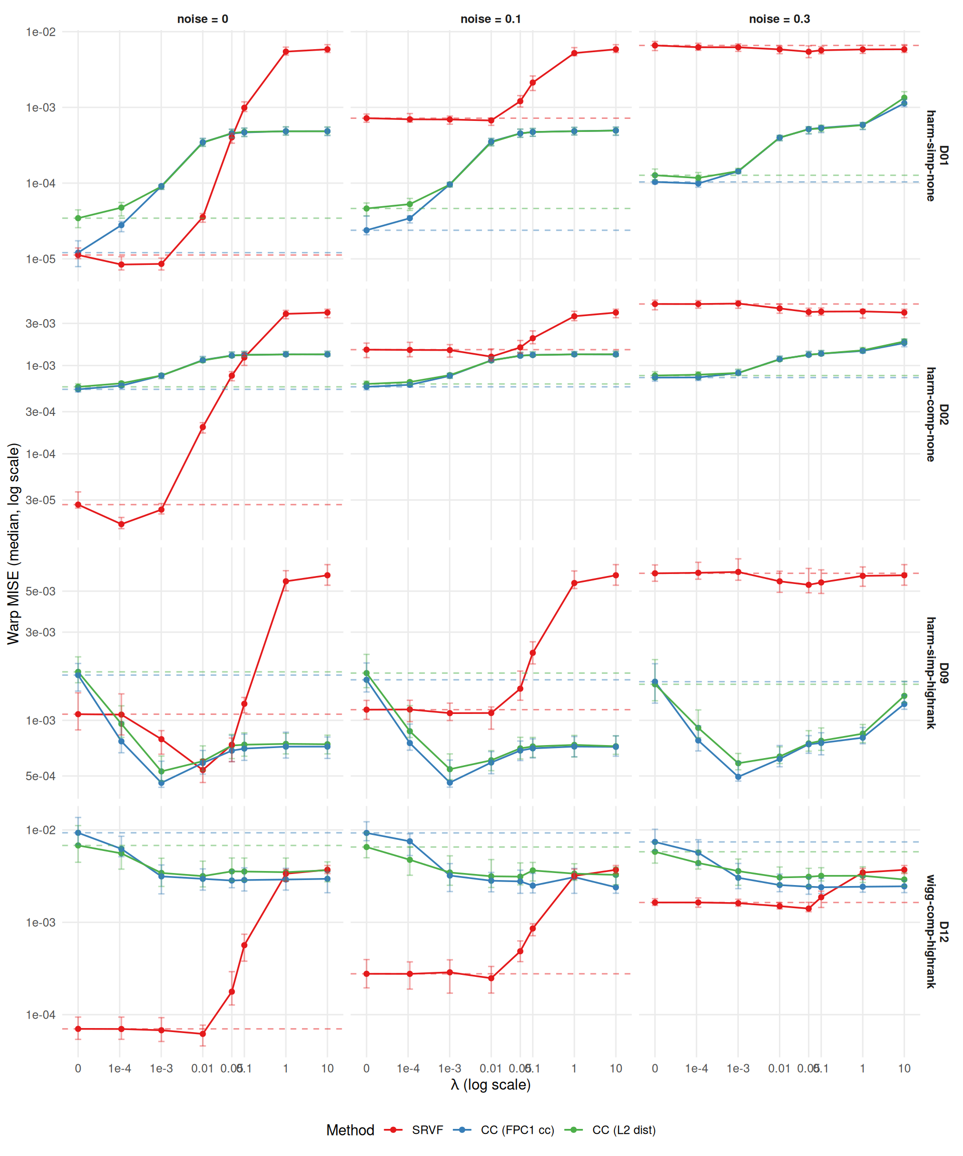

Same as above but for severity = 0.5.

2 Optimal Lambda

cat("## Optimal lambda per method x DGP x condition\n\n")

2.1 Optimal lambda per method x DGP x condition

opt_wide <- dcast(
  optimal[, .(method, dgp, severity, noise_sd, lambda)],
  method + dgp + severity ~ noise_sd,
  value.var = "lambda"
)
knitr::kable(opt_wide, caption = "Optimal lambda by method, DGP, and severity. Columns show noise levels.")

Optimal lambda by method, DGP, and severity. Columns show noise levels.

method	dgp	severity	0	0.1	0.3
srvf	D01	0.5	0.000	1e-02	5e-02
srvf	D01	1	0.001	0e+00	1e-01
srvf	D02	0.5	0.000	1e-02	1e+01
srvf	D02	1	0.000	0e+00	1e-01
srvf	D09	0.5	0.010	1e-03	5e-02
srvf	D09	1	0.001	0e+00	5e-02
srvf	D12	0.5	0.010	1e-02	5e-02
srvf	D12	1	0.000	0e+00	0e+00
cc_default	D01	0.5	0.000	0e+00	0e+00
cc_default	D01	1	0.000	0e+00	0e+00
cc_default	D02	0.5	0.000	0e+00	0e+00
cc_default	D02	1	0.000	0e+00	0e+00
cc_default	D09	0.5	0.001	1e-03	1e-03
cc_default	D09	1	0.001	1e-03	1e-03
cc_default	D12	0.5	0.050	1e+01	1e-01
cc_default	D12	1	1.000	1e+01	1e-02
cc_crit1	D01	0.5	0.000	0e+00	0e+00
cc_crit1	D01	1	0.001	1e-03	1e-03
cc_crit1	D02	0.5	0.000	0e+00	0e+00
cc_crit1	D02	1	0.001	1e-03	1e-03
cc_crit1	D09	0.5	0.001	1e-03	1e-03
cc_crit1	D09	1	0.001	1e-03	1e-03
cc_crit1	D12	0.5	0.010	5e-02	1e+01
cc_crit1	D12	1	1.000	1e+00	1e-01

# Check if optimal lambda shifts with noise
cat("\n## Does optimal lambda shift with noise?\n\n")

2.2 Does optimal lambda shift with noise?

for (m in levels(dt$method)) {
  sub <- optimal[method == m]
  # Most common optimal lambda per noise level (mode, not median — grid is discrete)
  by_noise <- sub[, .(
    mode_lambda = {
      tab <- table(lambda)
      as.numeric(names(tab)[which.max(tab)])
    },
    n_zero = sum(lambda == 0),
    n_total = .N
  ), by = noise_sd]
  cat(sprintf("- **%s**: most common optimal λ by noise: %s. ",
    mlabs[m],
    paste(sprintf("noise=%s → %g (%d/%d at λ=0)",
      by_noise$noise_sd, by_noise$mode_lambda,
      by_noise$n_zero, by_noise$n_total), collapse = "; ")))
  # Full frequency table across all conditions
  freq <- sub[, .N, by = lambda][order(lambda)]
  freq_txt <- paste(sprintf("%g: %d", freq$lambda, freq$N), collapse = ", ")
  cat(sprintf("Distribution: {%s}. ", freq_txt))
  # Flag boundary hits
  n_boundary <- sum(sub$lambda == max(sub$lambda))
  if (n_boundary > 0) {
    cat(sprintf("**%d/%d cells hit boundary (λ=%g).**",
      n_boundary, nrow(sub), max(sub$lambda)))
  }
  cat("\n")
}

• SRVF: most common optimal λ by noise: noise=0 → 0.0001 (0/8 at λ=0); noise=0.1 → 0.0001 (1/8 at λ=0); noise=0.3 → 0.05 (1/8 at λ=0). Distribution: {0: 2, 0.0001: 7, 0.001: 3, 0.01: 5, 0.05: 4, 0.1: 2, 10: 1}. 1/24 cells hit boundary (λ=10).
• CC (FPC1 cc): most common optimal λ by noise: noise=0 → 0 (2/8 at λ=0); noise=0.1 → 0 (2/8 at λ=0); noise=0.3 → 0.0001 (1/8 at λ=0). Distribution: {0: 5, 0.0001: 7, 0.001: 6, 0.01: 1, 0.05: 1, 0.1: 1, 1: 1, 10: 2}. 2/24 cells hit boundary (λ=10).
• CC (L2 dist): most common optimal λ by noise: noise=0 → 0.001 (2/8 at λ=0); noise=0.1 → 0.001 (2/8 at λ=0); noise=0.3 → 0.001 (1/8 at λ=0). Distribution: {0: 5, 0.0001: 1, 0.001: 12, 0.01: 1, 0.05: 1, 0.1: 1, 1: 2, 10: 1}. 1/24 cells hit boundary (λ=10).

3 Improvement from Penalization

How much does the best lambda improve over lambda=0?

Note: This is an oracle analysis — the optimal lambda is selected ex post from the same data used to evaluate it. Ratios \(\leq 1\) by construction (the baseline lambda=0 is always in the candidate set). The practical benefit of penalization depends on whether a good lambda can be selected a priori or via cross-validation.

min_ratio <- min(merged$ratio, na.rm = TRUE)

ggplot(merged,
  aes(x = interaction(noise_sd, severity, sep = " / sev="),
    y = interaction(dgp, method, sep = " : "),
    fill = ratio)) +
  geom_tile(color = "white") +
  geom_text(aes(label = sprintf("%.2f\n(λ=%g)", ratio, lambda)),
    size = 2.5) +
  scale_fill_gradient(
    low = "#2ca02c", high = "white",
    limits = c(min_ratio, 1),
    oob = scales::squish
  ) +
  labs(x = "noise / severity",
    y = "DGP : Method",
    fill = "MISE ratio\n(vs λ=0)") +
  theme_benchmark() +
  theme(axis.text.x = element_text(angle = 45, hjust = 1))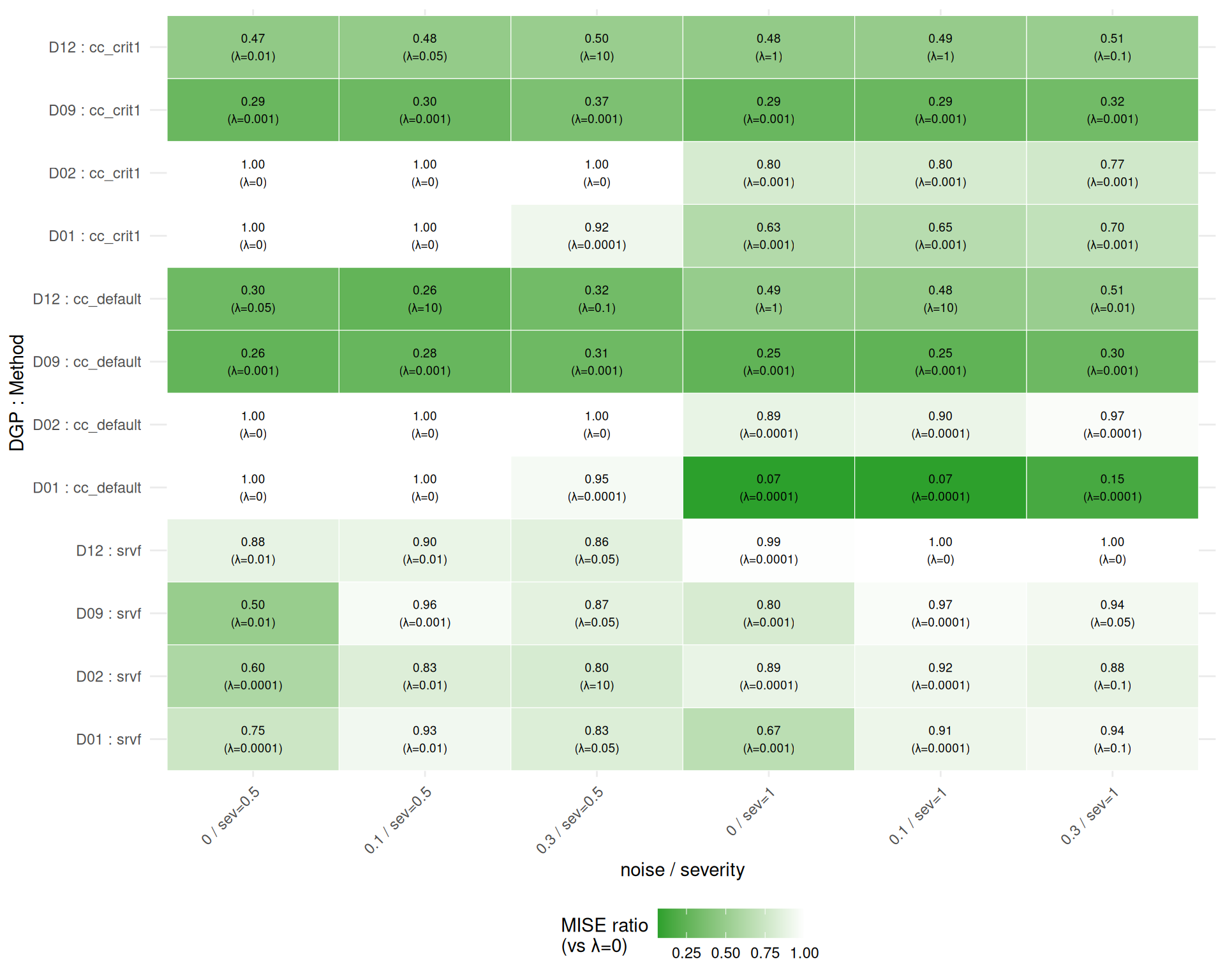

Improvement ratio: MISE(optimal lambda) / MISE(lambda=0). Values < 1 mean penalization helps; 1 means no gain. Ratios > 1 cannot occur because lambda=0 is in the candidate set.

cat("**Findings:**\n\n")

Findings:

ratio_by_method <- mean_se_table(merged, "ratio", "method")[order(mean)]
cat("Average improvement ratio across the 24 method-specific cells ",
  "(mean ± SE; lower is better):\n\n")

Average improvement ratio across the 24 method-specific cells (mean ± SE; lower is better):

for (i in seq_len(nrow(ratio_by_method))) {
  r <- ratio_by_method[i]
  cat(sprintf("- **%s**: %s (n=%d)\n",
    mlabs[r$method], fmt_mean_se(r$mean, r$se), r$n))
}

• CC (FPC1 cc): 0.54 ± 0.07 (n=24)
• CC (L2 dist): 0.63 ± 0.05 (n=24)
• SRVF: 0.86 ± 0.03 (n=24)

cat("\n")

# Biggest winners
big_win <- merged[ratio < 0.8][order(ratio)]
if (nrow(big_win) > 0) {
  cat("Cases where penalization improves MISE by >20%:\n\n")
  for (i in seq_len(min(nrow(big_win), 10))) {
    r <- big_win[i]
    cat(sprintf("- %s on %s (noise=%s, sev=%s): %.0f%% improvement at λ=%g\n",
      mlabs[r$method], r$dgp, r$noise_sd, r$severity,
      100 * (1 - r$ratio), r$lambda))
  }
}

Cases where penalization improves MISE by >20%:

• CC (FPC1 cc) on D01 (noise=0, sev=1): 93% improvement at λ=0.0001
• CC (FPC1 cc) on D01 (noise=0.1, sev=1): 93% improvement at λ=0.0001
• CC (FPC1 cc) on D01 (noise=0.3, sev=1): 85% improvement at λ=0.0001
• CC (FPC1 cc) on D09 (noise=0.1, sev=1): 75% improvement at λ=0.001
• CC (FPC1 cc) on D09 (noise=0, sev=1): 75% improvement at λ=0.001
• CC (FPC1 cc) on D12 (noise=0.1, sev=0.5): 74% improvement at λ=10
• CC (FPC1 cc) on D09 (noise=0, sev=0.5): 74% improvement at λ=0.001
• CC (FPC1 cc) on D09 (noise=0.1, sev=0.5): 72% improvement at λ=0.001
• CC (L2 dist) on D09 (noise=0, sev=1): 71% improvement at λ=0.001
• CC (L2 dist) on D09 (noise=0.1, sev=1): 71% improvement at λ=0.001

cat("\n")

4 CC Criterion Comparison

Does cc_crit1 respond differently to lambda than cc_default?

# Check whether severity=0.5 patterns differ qualitatively
fda_both <- dt[failure == FALSE & method %in% c("cc_default", "cc_crit1")]
fda_agg_both <- fda_both[,
  .(mise = median(warp_mise, na.rm = TRUE)),
  by = .(method, dgp, noise_sd, severity, lambda)
]
# Correlation of MISE profiles across severity
cor_default <- cor(
  fda_agg_both[method == "cc_default" & severity == "0.5", mise],
  fda_agg_both[method == "cc_default" & severity == "1", mise],
  use = "complete.obs"
)
cor_crit1 <- cor(
  fda_agg_both[method == "cc_crit1" & severity == "0.5", mise],
  fda_agg_both[method == "cc_crit1" & severity == "1", mise],
  use = "complete.obs"
)
cat(sprintf(
  "Results shown for severity=1.0. MISE profiles are highly correlated across severities (r=%.2f for cc_default, r=%.2f for cc_crit1); severity=0.5 patterns are qualitatively similar.\n\n",
  cor_default, cor_crit1))

Results shown for severity=1.0. MISE profiles are highly correlated across severities (r=0.95 for cc_default, r=0.99 for cc_crit1); severity=0.5 patterns are qualitatively similar.

fda_dt <- dt[failure == FALSE & method %in% c("cc_default", "cc_crit1")]
fda_agg <- aggregate_median_iqr(
  dt = fda_dt[severity == "1"],
  metric = "warp_mise",
  by = c("method", "dgp", "noise_sd", "lambda"),
  value_name = "mise"
)

ggplot(fda_agg,
  aes(x = lambda + 1e-5, y = mise, color = method)) +
  geom_line(linewidth = 0.8) +
  geom_point(size = 2) +
  geom_errorbar(aes(ymin = q25, ymax = q75), width = 0.15, alpha = 0.35) +
  facet_grid(dgp ~ noise_sd,
    scales = "free_y",
    labeller = labeller(
      noise_sd = function(x) paste0("noise = ", x),
      dgp = dlabs)) +
  scale_x_log10(
    breaks = c(1e-5, 1e-4, 1e-3, 0.01, 0.05, 0.1, 1, 10),
    labels = c("0", "1e-4", "1e-3", "0.01", "0.05", "0.1", "1", "10")) +
  scale_color_manual(values = mcols, labels = mlabs) +
  scale_y_log10() +
  labs(x = expression(lambda ~ "(log scale)"),
    y = "Warp MISE (median, log scale)",
    color = "Method") +
  theme_benchmark() +
  theme(legend.position = "bottom")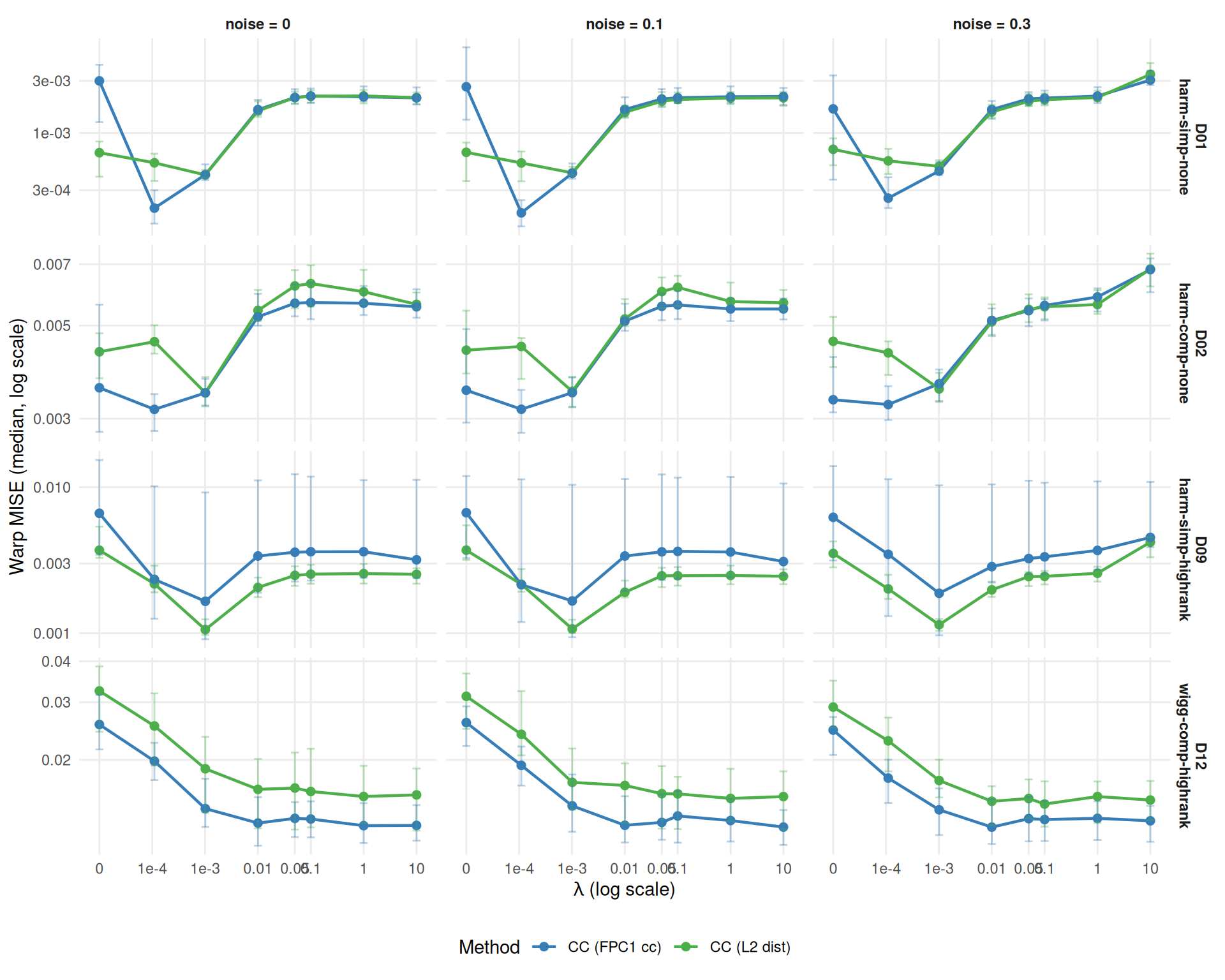

Direct comparison of cc_default vs cc_crit1 MISE across lambda values. Points show medians and vertical bars show IQRs in each DGP × noise panel at severity=1.0.

# Compare optimal lambdas for the two CC methods
fda_opt <- optimal[method %in% c("cc_default", "cc_crit1")]
fda_comp <- dcast(
  fda_opt[, .(method, dgp, noise_sd, severity, lambda, mise)],
  dgp + noise_sd + severity ~ method,
  value.var = list("lambda", "mise")
)

cat("**CC criterion comparison:**\n\n")

CC criterion comparison:

# Paired comparison: how often is crit1's optimal lambda higher/lower/equal?
fda_comp[, crit1_higher := lambda_cc_crit1 > lambda_cc_default]
fda_comp[, crit1_lower := lambda_cc_crit1 < lambda_cc_default]
fda_comp[, crit1_equal := lambda_cc_crit1 == lambda_cc_default]
n_higher <- sum(fda_comp$crit1_higher, na.rm = TRUE)
n_lower <- sum(fda_comp$crit1_lower, na.rm = TRUE)
n_equal <- sum(fda_comp$crit1_equal, na.rm = TRUE)
n_comp <- nrow(fda_comp)
cat(sprintf(
  "- Paired comparison of optimal λ: cc_crit1 higher in %d/%d, lower in %d/%d, equal in %d/%d cells.\n",
  n_higher, n_comp, n_lower, n_comp, n_equal, n_comp))

• Paired comparison of optimal λ: cc_crit1 higher in 8/24, lower in 3/24, equal in 13/24 cells.

# Which criterion wins at its own optimal lambda?
fda_comp[, crit1_wins := mise_cc_crit1 < mise_cc_default]
cat(sprintf("- At each method's optimal lambda, cc_crit1 wins in %d/%d conditions.\n",
  sum(fda_comp$crit1_wins, na.rm = TRUE), nrow(fda_comp)))

• At each method’s optimal lambda, cc_crit1 wins in 3/24 conditions.

fda_comp[, mise_gap := mise_cc_crit1 - mise_cc_default]
gap_summary <- mean_se_table(fda_comp, "mise_gap", character())[1]
cat(sprintf(
  "- At each method's own optimum, the average MISE difference (crit1 - default) is %s.\n",
  fmt_mean_se(gap_summary$mean, gap_summary$se, digits = 3)
))

• At each method’s own optimum, the average MISE difference (crit1 - default) is 0.000 ± 0.000.

cat("\n")

5 SRVF Lambda Behavior

SRVF’s lambda response is expected to differ qualitatively from CC methods.

srvf_both <- dt[failure == FALSE & method == "srvf"]
srvf_agg_both <- srvf_both[,
  .(mise = median(warp_mise, na.rm = TRUE)),
  by = .(dgp, noise_sd, severity, lambda)
]
cor_srvf <- cor(
  srvf_agg_both[severity == "0.5", mise],
  srvf_agg_both[severity == "1", mise],
  use = "complete.obs"
)
cat(sprintf(
  "Results shown for severity=1.0. SRVF MISE profiles across severities are highly correlated (r=%.2f); severity=0.5 patterns are qualitatively similar.\n\n",
  cor_srvf))

Results shown for severity=1.0. SRVF MISE profiles across severities are highly correlated (r=0.94); severity=0.5 patterns are qualitatively similar.

srvf_agg <- dt[failure == FALSE & method == "srvf" & severity == "1",
  .(mise = median(warp_mise, na.rm = TRUE),
    q25 = quantile(warp_mise, 0.25, na.rm = TRUE),
    q75 = quantile(warp_mise, 0.75, na.rm = TRUE)),
  by = .(dgp, noise_sd, lambda)
]

ggplot(srvf_agg,
  aes(x = lambda + 1e-5, y = mise, color = noise_sd)) +
  geom_line(linewidth = 0.8) +
  geom_point(size = 2) +
  geom_ribbon(aes(ymin = q25, ymax = q75, fill = noise_sd),
    alpha = 0.15, color = NA) +
  facet_wrap(~dgp, scales = "free_y", labeller = as_labeller(dlabs)) +
  scale_x_log10(
    breaks = c(1e-5, 1e-4, 1e-3, 0.01, 0.05, 0.1, 1, 10),
    labels = c("0", "1e-4", "1e-3", "0.01", "0.05", "0.1", "1", "10")) +
  scale_color_brewer(palette = "Set1") +
  scale_fill_brewer(palette = "Set1") +
  scale_y_log10() +
  labs(x = expression(lambda ~ "(log scale)"),
    y = "Warp MISE (median ± IQR, log scale)",
    color = "Noise", fill = "Noise") +
  theme_benchmark() +
  theme(legend.position = "bottom")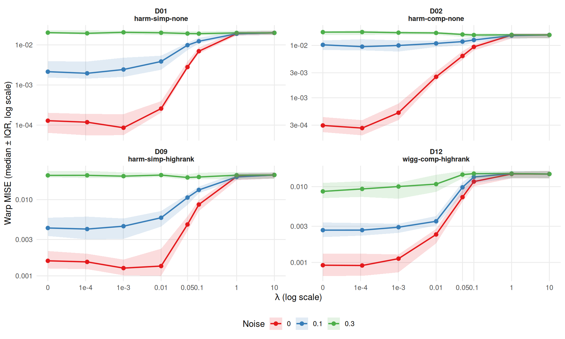

SRVF warp MISE vs lambda across all DGPs and noise levels (severity=1.0). The lambda response ranges from ‘U-shape’ (lambda helps) to ‘monotone increasing’ (lambda only hurts).

srvf_opt <- optimal[method == "srvf"]
cat("**SRVF lambda findings:**\n\n")

SRVF lambda findings:

for (d in levels(dt$dgp)) {
  sub <- srvf_opt[dgp == d]
  lambdas <- sub[, .(noise_sd, lambda, mise)]
  cat(sprintf("- **%s** (%s): optimal λ = %s\n",
    d, dlabs[d],
    paste(sprintf("%g (noise=%s)", lambdas$lambda, lambdas$noise_sd),
      collapse = ", ")))
}

• D01 (D01 harm-simp-none): optimal λ = 0.0001 (noise=0), 0.01 (noise=0.1), 0.05 (noise=0.3), 0.001 (noise=0), 0.0001 (noise=0.1), 0.1 (noise=0.3)
• D02 (D02 harm-comp-none): optimal λ = 0.0001 (noise=0), 0.01 (noise=0.1), 10 (noise=0.3), 0.0001 (noise=0), 0.0001 (noise=0.1), 0.1 (noise=0.3)
• D09 (D09 harm-simp-highrank): optimal λ = 0.01 (noise=0), 0.001 (noise=0.1), 0.05 (noise=0.3), 0.001 (noise=0), 0.0001 (noise=0.1), 0.05 (noise=0.3)
• D12 (D12 wigg-comp-highrank): optimal λ = 0.01 (noise=0), 0.01 (noise=0.1), 0.05 (noise=0.3), 0.0001 (noise=0), 0 (noise=0.1), 0 (noise=0.3)

cat("\n")

# Does lambda ever help SRVF substantially?
srvf_merged <- merged[method == "srvf"]
helps <- srvf_merged[ratio < 0.9]
if (nrow(helps) > 0) {
  cat(sprintf("Lambda helps SRVF (>10%% improvement) in %d/%d conditions:\n",
    nrow(helps), nrow(srvf_merged)))
  for (i in seq_len(nrow(helps))) {
    r <- helps[i]
    cat(sprintf("  - %s noise=%s sev=%s: %.0f%% at λ=%g\n",
      r$dgp, r$noise_sd, r$severity, 100*(1-r$ratio), r$lambda))
  }
} else {
  cat("Lambda does not substantially help SRVF (>10%) in any condition.\n")
}

Lambda helps SRVF (>10% improvement) in 14/24 conditions: - D01 noise=0 sev=0.5: 25% at λ=0.0001 - D01 noise=0 sev=1: 33% at λ=0.001 - D01 noise=0.3 sev=0.5: 17% at λ=0.05 - D02 noise=0 sev=0.5: 40% at λ=0.0001 - D02 noise=0 sev=1: 11% at λ=0.0001 - D02 noise=0.1 sev=0.5: 17% at λ=0.01 - D02 noise=0.3 sev=0.5: 20% at λ=10 - D02 noise=0.3 sev=1: 12% at λ=0.1 - D09 noise=0 sev=0.5: 50% at λ=0.01 - D09 noise=0 sev=1: 20% at λ=0.001 - D09 noise=0.3 sev=0.5: 13% at λ=0.05 - D12 noise=0 sev=0.5: 12% at λ=0.01 - D12 noise=0.1 sev=0.5: 10% at λ=0.01 - D12 noise=0.3 sev=0.5: 14% at λ=0.05

srvf_ratio_summary <- mean_se_table(srvf_merged, "ratio", character())[1]
cat(sprintf(
  "Average SRVF improvement ratio across cells: %s (n=%d).\n",
  fmt_mean_se(srvf_ratio_summary$mean, srvf_ratio_summary$se),
  srvf_ratio_summary$n
))

Average SRVF improvement ratio across cells: 0.86 ± 0.03 (n=24).

cat("\n")

6 Template Quality under Penalization

Does lambda affect template estimation quality?

tmpl_both <- dt[failure == FALSE,
  .(tmise = median(template_mise, na.rm = TRUE)),
  by = .(method, dgp, noise_sd, severity, lambda)
]
cor_tmpl <- cor(
  tmpl_both[severity == "0.5", tmise],
  tmpl_both[severity == "1", tmise],
  use = "complete.obs"
)
cat(sprintf(
  "Results shown for severity=1.0. Template MISE profiles across severities are highly correlated (r=%.2f); severity=0.5 patterns are qualitatively similar.\n\n",
  cor_tmpl))

Results shown for severity=1.0. Template MISE profiles across severities are highly correlated (r=0.87); severity=0.5 patterns are qualitatively similar.

tmpl_agg <- aggregate_median_iqr(
  dt = dt[failure == FALSE & severity == "1"],
  metric = "template_mise",
  by = c("method", "dgp", "noise_sd", "lambda"),
  value_name = "tmise"
)

ggplot(tmpl_agg,
  aes(x = lambda + 1e-5, y = tmise, color = method)) +
  geom_line(linewidth = 0.6) +
  geom_point(size = 1.5) +
  geom_errorbar(aes(ymin = q25, ymax = q75), width = 0.15, alpha = 0.35) +
  facet_grid(dgp ~ noise_sd,
    scales = "free_y",
    labeller = labeller(
      noise_sd = function(x) paste0("noise = ", x),
      dgp = dlabs)) +
  scale_x_log10(
    breaks = c(1e-5, 1e-4, 1e-3, 0.01, 0.05, 0.1, 1, 10),
    labels = c("0", "1e-4", "1e-3", "0.01", "0.05", "0.1", "1", "10")) +
  scale_color_manual(values = mcols, labels = mlabs) +
  scale_y_log10() +
  labs(x = expression(lambda ~ "(log scale)"),
    y = "Template MISE (median, log scale)",
    color = "Method") +
  theme_benchmark() +
  theme(legend.position = "bottom")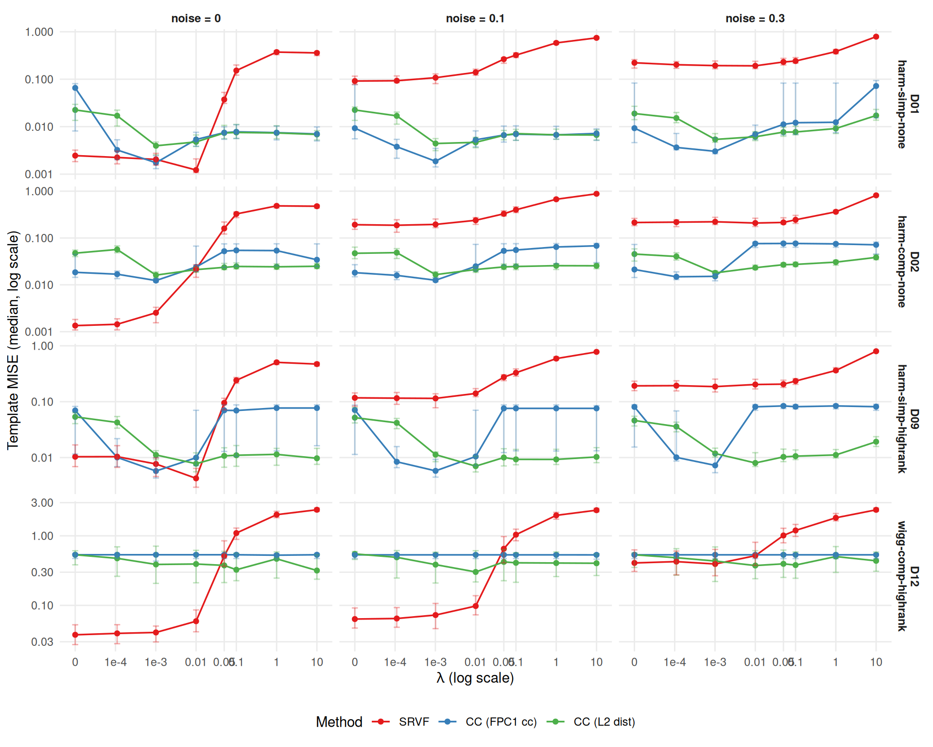

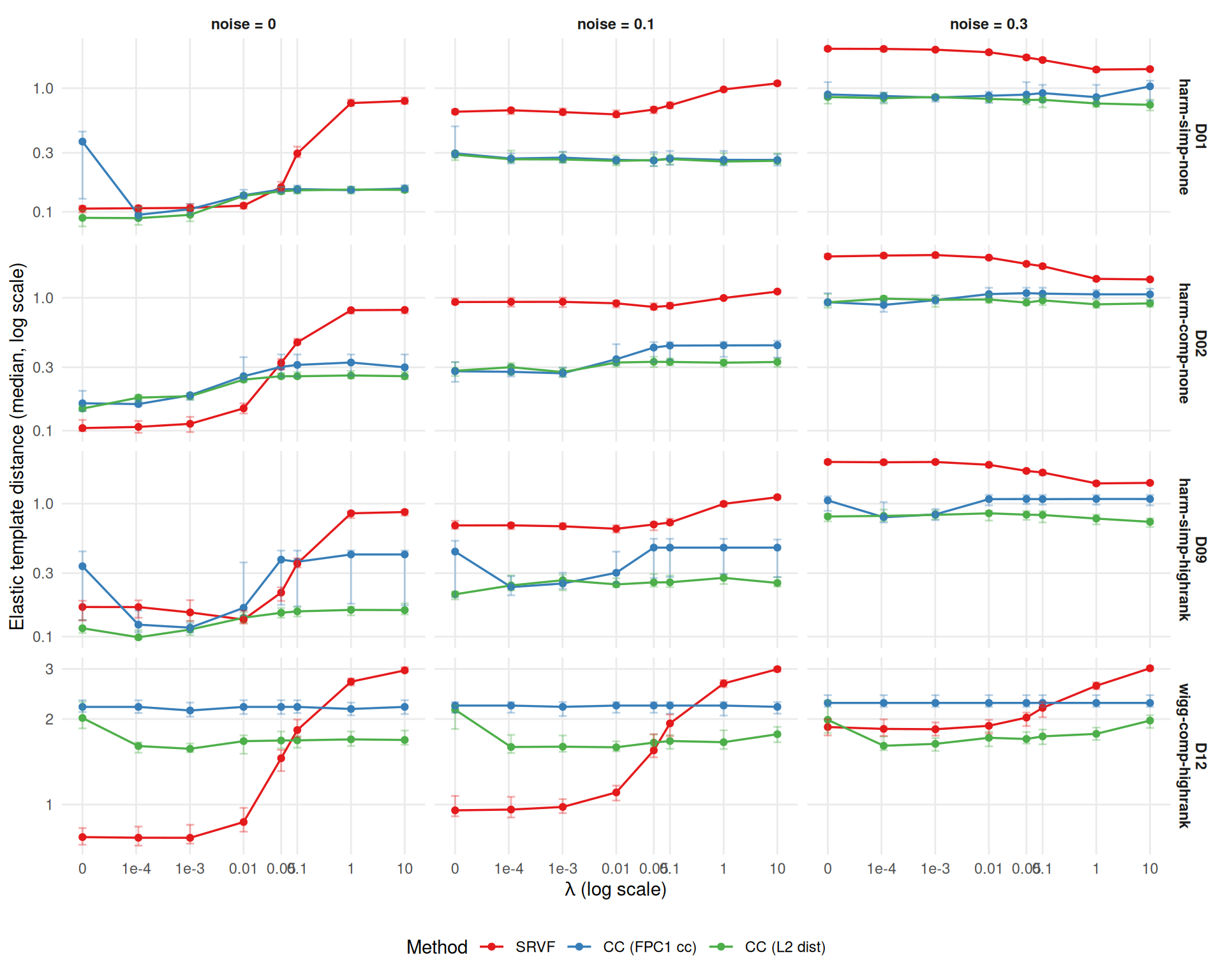
Template MISE vs lambda. Points show medians and vertical bars show IQRs. Penalization can improve template estimation by smoothing the iterative estimation.

has_elastic_b <- "template_elastic_dist" %in% names(dt) &&
  any(!is.na(dt$template_elastic_dist))

if (has_elastic_b) {
  edist_agg <- aggregate_median_iqr(
    dt = dt[failure == FALSE & severity == "1" &
        !is.na(template_elastic_dist)],
    metric = "template_elastic_dist",
    by = c("method", "dgp", "noise_sd", "lambda"),
    value_name = "edist"
  )

  ggplot(edist_agg,
    aes(x = lambda + 1e-5, y = edist, color = method)) +
    geom_line(linewidth = 0.6) +
    geom_point(size = 1.5) +
    geom_errorbar(aes(ymin = q25, ymax = q75), width = 0.15, alpha = 0.35) +
    facet_grid(dgp ~ noise_sd,
      scales = "free_y",
      labeller = labeller(
        noise_sd = function(x) paste0("noise = ", x),
        dgp = dlabs)) +
    scale_x_log10(
      breaks = c(1e-5, 1e-4, 1e-3, 0.01, 0.05, 0.1, 1, 10),
      labels = c("0", "1e-4", "1e-3", "0.01", "0.05", "0.1", "1", "10")) +
    scale_color_manual(values = mcols, labels = mlabs) +
    scale_y_log10() +
    labs(x = expression(lambda ~ "(log scale)"),
      y = "Elastic template distance (median, log scale)",
      color = "Method") +
    theme_benchmark() +
    theme(legend.position = "bottom")
} else {
  cat("*Elastic template distance not available in Study B results.*")
}

Elastic (Fisher-Rao) template distance vs lambda. Points show medians and vertical bars show IQRs. This reparameterization-invariant metric isolates template shape quality from phase shifts.

if (has_elastic_b) {
  # Optimize each template metric separately to avoid mixed-target bias
  tmpl_base <- dt[failure == FALSE & lambda == 0 & severity == "1",
    .(tmise_base = median(template_mise, na.rm = TRUE),
      edist_base = median(template_elastic_dist, na.rm = TRUE)),
    by = .(method, dgp, noise_sd)]
  tmpl_by_lambda <- dt[failure == FALSE & severity == "1" &
      !is.na(template_elastic_dist),
    .(tmise = median(template_mise, na.rm = TRUE),
      edist = median(template_elastic_dist, na.rm = TRUE)),
    by = .(method, dgp, noise_sd, lambda)]

  # Best lambda for elastic distance
  best_edist <- tmpl_by_lambda[,
    .SD[which.min(edist)],
    by = .(method, dgp, noise_sd)]
  edist_comp <- merge(best_edist, tmpl_base, by = c("method", "dgp", "noise_sd"))
  edist_comp[, edist_ratio := edist / edist_base]

  # Best lambda for template MISE (optimized independently)
  best_tmise <- tmpl_by_lambda[,
    .SD[which.min(tmise)],
    by = .(method, dgp, noise_sd)]
  tmise_comp <- merge(best_tmise, tmpl_base, by = c("method", "dgp", "noise_sd"))
  tmise_comp[, tmise_ratio := tmise / tmise_base]

  n_edist_helps <- sum(edist_comp$edist_ratio < 0.9)
  n_tmise_helps <- sum(tmise_comp$tmise_ratio < 0.9)
  cat(sprintf(
    "**Template quality under penalization** (each metric optimized at its own best λ): elastic template distance improves >10%% in %d/%d cells; template MISE improves >10%% in %d/%d cells. ",
    n_edist_helps, nrow(edist_comp), n_tmise_helps, nrow(tmise_comp)))

  # Which method benefits most for template shape?
  avg_edist <- edist_comp[, .(mean_ratio = mean(edist_ratio, na.rm = TRUE)),
    by = method]
  best_tmpl_m <- avg_edist[which.min(mean_ratio)]
  edist_method_summary <- mean_se_table(edist_comp, "edist_ratio", "method")
  best_tmpl_summary <- edist_method_summary[method == best_tmpl_m$method]
  cat(sprintf(
    "%s benefits most for template *shape* (mean elastic distance ratio %s).\n\n",
    mlabs[best_tmpl_m$method],
    fmt_mean_se(best_tmpl_summary$mean, best_tmpl_summary$se)
  ))
}

Template quality under penalization (each metric optimized at its own best λ): elastic template distance improves >10% in 15/36 cells; template MISE improves >10% in 24/36 cells. CC (FPC1 cc) benefits most for template shape (mean elastic distance ratio 0.80 ± 0.08).

7 Alignment Error under Penalization

Alignment error measures how well registered curves match the true pre-warp curves: \(\text{mean}_i \int (\hat{x}_i^{\text{aligned}} - \tilde{x}_i)^2\,dt\). This captures the practical downstream impact of registration quality, complementing the warp MISE.

ae_agg <- dt[failure == FALSE,
  .(ae = median(alignment_error, na.rm = TRUE),
    q25 = quantile(alignment_error, 0.25, na.rm = TRUE),
    q75 = quantile(alignment_error, 0.75, na.rm = TRUE)),
  by = .(method, dgp, noise_sd, severity, lambda)
]

ae_baseline <- ae_agg[lambda == 0, .(method, dgp, noise_sd, severity, base = ae)]

ggplot(ae_agg[severity == "1"],
  aes(x = lambda + 1e-5, y = ae, color = method)) +
  geom_line(linewidth = 0.6) +
  geom_point(size = 1.5) +
  geom_errorbar(aes(ymin = q25, ymax = q75), width = 0.15, alpha = 0.4) +
  geom_hline(data = ae_baseline[severity == "1"],
    aes(yintercept = base, color = method),
    linetype = "dashed", alpha = 0.5) +
  facet_grid(dgp ~ noise_sd,
    scales = "free_y",
    labeller = labeller(
      noise_sd = function(x) paste0("noise = ", x),
      dgp = dlabs)) +
  scale_x_log10(
    breaks = c(1e-5, 1e-4, 1e-3, 0.01, 0.05, 0.1, 1, 10),
    labels = c("0", "1e-4", "1e-3", "0.01", "0.05", "0.1", "1", "10")) +
  scale_color_manual(values = mcols, labels = mlabs) +
  scale_y_log10() +
  labs(x = expression(lambda ~ "(log scale)"),
    y = "Alignment error (median, log scale)",
    color = "Method") +
  theme_benchmark() +
  theme(legend.position = "bottom")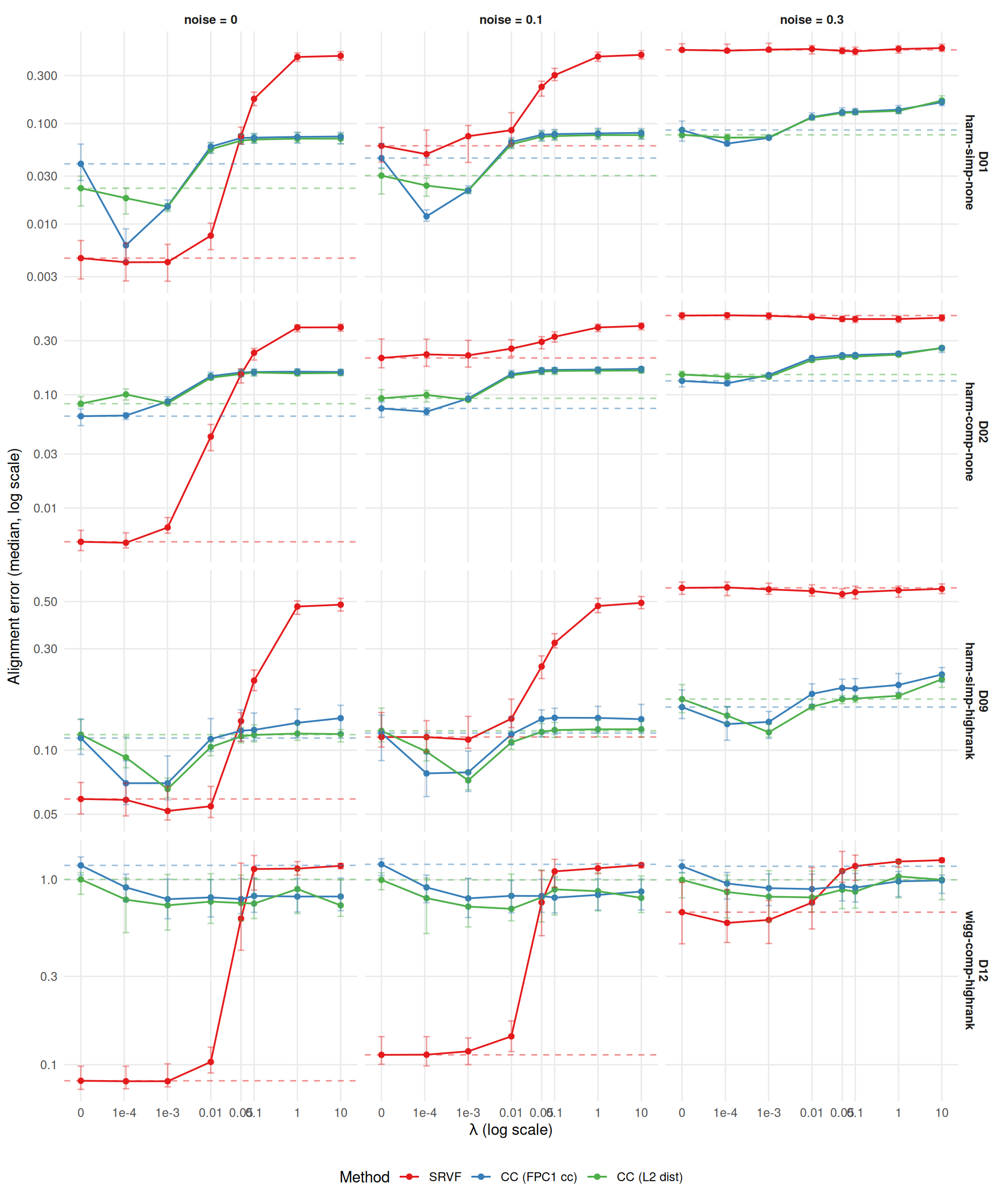

Median alignment error vs lambda for each method, faceted by DGP (rows) and noise level (columns). Dashed horizontal line = lambda=0 baseline.

cat("**Alignment error: optimal lambda and improvement**\n\n")

Alignment error: optimal lambda and improvement

# How often does lambda > 0 help alignment error?
n_helps_ae <- nrow(ae_merged[ratio < 0.95])
n_total_ae <- nrow(ae_merged)
cat(sprintf("- Lambda > 0 improves alignment error by >5%% in %d/%d (%.0f%%) cells.\n",
  n_helps_ae, n_total_ae, 100 * n_helps_ae / n_total_ae))

• Lambda > 0 improves alignment error by >5% in 42/72 (58%) cells.

# Does alignment error agree with warp MISE on optimal lambda?
agree <- sum(lambda_comp$agree)
cat(sprintf("- Optimal lambda for alignment error agrees with warp MISE in %d/%d (%.0f%%) cells.\n",
  agree, nrow(lambda_comp), 100 * agree / nrow(lambda_comp)))

• Optimal lambda for alignment error agrees with warp MISE in 42/72 (58%) cells.

# Correlation between alignment error and warp MISE improvement ratios
warp_merged_sub <- merged[, .(method, dgp, noise_sd, severity, warp_ratio = ratio)]
ae_merged_sub <- ae_merged[, .(method, dgp, noise_sd, severity, ae_ratio = ratio)]
both <- merge(warp_merged_sub, ae_merged_sub,
  by = c("method", "dgp", "noise_sd", "severity"))
r_improvement <- cor(both$warp_ratio, both$ae_ratio, use = "complete.obs")
cat(sprintf("- Correlation between warp MISE and alignment error improvement ratios: r = %.2f.\n",
  r_improvement))

• Correlation between warp MISE and alignment error improvement ratios: r = 0.86.

ae_ratio_summary <- mean_se_table(ae_merged, "ratio", "method")[order(mean)]
cat("Average alignment-error improvement ratio across the 24 method-specific cells ",
  "(mean ± SE):\n\n")

Average alignment-error improvement ratio across the 24 method-specific cells (mean ± SE):

for (i in seq_len(nrow(ae_ratio_summary))) {
  r <- ae_ratio_summary[i]
  cat(sprintf("- **%s**: %s (n=%d)\n",
    mlabs[r$method], fmt_mean_se(r$mean, r$se), r$n))
}

• CC (FPC1 cc): 0.72 ± 0.05 (n=24)
• CC (L2 dist): 0.83 ± 0.03 (n=24)
• SRVF: 0.93 ± 0.01 (n=24)

cat("\n")

# Biggest improvement
biggest_ae <- ae_merged[which.min(ratio)]
cat(sprintf("- Largest alignment error improvement: %s on %s (noise=%s, sev=%s): %.0f%% at λ=%g.\n\n",
  mlabs[biggest_ae$method], biggest_ae$dgp, biggest_ae$noise_sd, biggest_ae$severity,
  100 * (1 - biggest_ae$ratio), biggest_ae$lambda))

• Largest alignment error improvement: CC (FPC1 cc) on D01 (noise=0, sev=1): 85% at λ=0.0001.

if (r_improvement > 0.9) {
  cat("The two metrics respond nearly identically to penalization — the same lambdas ",
    "that improve warp recovery also improve alignment quality.\n")
} else if (r_improvement > 0.7) {
  cat("The metrics are strongly correlated but not identical — in some cells, the ",
    "lambda that minimizes warp MISE is not optimal for alignment error.\n")
} else {
  cat("The metrics show moderate agreement — penalization affects warp recovery ",
    "and alignment quality somewhat differently.\n")
}

The metrics are strongly correlated but not identical — in some cells, the lambda that minimizes warp MISE is not optimal for alignment error.

8 Summary

# Summary table: best lambda and improvement per method x DGP
summary_dt <- copy(merged)
summary_dt[, improvement := sprintf("%.0f%%", 100 * (1 - mise / base_mise))]
summary_dt[, cell := sprintf("λ=%g (%s)", lambda, improvement)]

summary_wide <- dcast(
  summary_dt[severity == "1", .(method, dgp, noise_sd, cell)],
  method + dgp ~ noise_sd,
  value.var = "cell"
)

cat("## Optimal lambda and improvement at severity=1.0\n\n")

8.1 Optimal lambda and improvement at severity=1.0

knitr::kable(
  summary_wide[order(method, dgp)],
  caption = "Optimal lambda and MISE improvement vs lambda=0, by method × DGP × noise (severity=1.0)."
)

Optimal lambda and MISE improvement vs lambda=0, by method × DGP × noise (severity=1.0).

method	dgp	0	0.1	0.3
srvf	D01	λ=0.001 (33%)	λ=0.0001 (9%)	λ=0.1 (6%)
srvf	D02	λ=0.0001 (11%)	λ=0.0001 (8%)	λ=0.1 (12%)
srvf	D09	λ=0.001 (20%)	λ=0.0001 (3%)	λ=0.05 (6%)
srvf	D12	λ=0.0001 (1%)	λ=0 (0%)	λ=0 (0%)
cc_default	D01	λ=0.0001 (93%)	λ=0.0001 (93%)	λ=0.0001 (85%)
cc_default	D02	λ=0.0001 (11%)	λ=0.0001 (10%)	λ=0.0001 (3%)
cc_default	D09	λ=0.001 (75%)	λ=0.001 (75%)	λ=0.001 (70%)
cc_default	D12	λ=1 (51%)	λ=10 (52%)	λ=0.01 (49%)
cc_crit1	D01	λ=0.001 (37%)	λ=0.001 (35%)	λ=0.001 (30%)
cc_crit1	D02	λ=0.001 (20%)	λ=0.001 (20%)	λ=0.001 (23%)
cc_crit1	D09	λ=0.001 (71%)	λ=0.001 (71%)	λ=0.001 (68%)
cc_crit1	D12	λ=1 (52%)	λ=1 (51%)	λ=0.1 (49%)

cat("## Key takeaways\n\n")

8.2 Key takeaways

cat("*Note: statistics below pool both severities unless stated otherwise.*\n\n")

Note: statistics below pool both severities unless stated otherwise.

# Count how often lambda > 0 is optimal
n_helps <- nrow(optimal[lambda > 0])
n_total <- nrow(optimal)
cat(sprintf("- Lambda > 0 is optimal in %d/%d (%.0f%%) of method × DGP × condition cells.\n",
  n_helps, n_total, 100 * n_helps / n_total))

• Lambda > 0 is optimal in 60/72 (83%) of method × DGP × condition cells.

# Severity breakdown for lambda > 0
for (s in levels(optimal$severity)) {
  sub <- optimal[severity == s]
  n_h <- nrow(sub[lambda > 0])
  n_t <- nrow(sub)
  cat(sprintf("  - Severity %s: %d/%d (%.0f%%)\n", s, n_h, n_t, 100 * n_h / n_t))
}

• Severity 0.5: 26/36 (72%)
• Severity 1: 34/36 (94%)

# Biggest beneficiary
biggest <- merged[which.min(ratio)]
cat(sprintf("- Largest improvement: %s on %s (noise=%s, sev=%s) — %.0f%% at λ=%g.\n",
  mlabs[biggest$method], biggest$dgp, biggest$noise_sd, biggest$severity,
  100 * (1 - biggest$ratio), biggest$lambda))

• Largest improvement: CC (FPC1 cc) on D01 (noise=0, sev=1) — 93% at λ=0.0001.

# Method that benefits most on average
avg_by_method <- mean_se_table(merged, "ratio", "method")
best_method <- avg_by_method[which.min(mean)]
cat(sprintf("- Method benefiting most from penalization on average: %s (mean ratio %.2f).\n",
  mlabs[best_method$method], best_method$mean))

• Method benefiting most from penalization on average: CC (FPC1 cc) (mean ratio 0.54).

# Severity breakdown for mean improvement ratio
cat("- Mean improvement ratio by method and severity:\n")

• Mean improvement ratio by method and severity:

avg_by_method_sev <- mean_se_table(merged, "ratio", c("method", "severity"))
for (i in seq_len(nrow(avg_by_method_sev))) {
  r <- avg_by_method_sev[i]
  cat(sprintf("  - %s, severity %s: %s\n",
    mlabs[r$method], r$severity, fmt_mean_se(r$mean, r$se)))
}

• SRVF, severity 0.5: 0.81 ± 0.04
• SRVF, severity 1: 0.91 ± 0.03
• CC (FPC1 cc), severity 0.5: 0.64 ± 0.11
• CC (FPC1 cc), severity 1: 0.44 ± 0.09
• CC (L2 dist), severity 0.5: 0.69 ± 0.09
• CC (L2 dist), severity 1: 0.56 ± 0.06

cat("\n")