Study A: Main Results

Registration Benchmark v2

Setup

Code

library(ggplot2)
library(data.table)
library(patchwork)
library(car)

base_dir <- here::here()
source(file.path(base_dir, "sim-analyze.R"))

mcols <- method_colors()
mlabs <- method_labels()
dlabs <- dgp_short_labels()
ddesc <- dgp_desc_labels()

Code

dt <- load_study_a()

Study A compares 5 registration methods across 15 DGPs in a crossed design: 15 DGPs \(\times\) 2 severity (0.5, 1.0) \(\times\) 3 noise (0, 0.1, 0.3) \(\times\) 5 methods = 450 cells \(\times\) 100 reps = 45,000 runs.

The DGP design is not full factorial (15 of 24 possible template \(\times\) warp \(\times\) amplitude combinations), but enables paired comparisons that vary exactly one factor while holding the other two constant.

Code

knitr::kable(
  dgp_factors(),
  caption = "DGP factor structure. 15 DGPs spanning 2 templates, 3 warp types, 4 amplitude types."
)

DGP factor structure. 15 DGPs spanning 2 templates, 3 warp types, 4 amplitude types.
dgp	template	warp_type	amplitude
D01	harmonic	simple	none
D02	harmonic	complex	none
D03	wiggly	complex	none
D04	harmonic	affine	none
D05	harmonic	simple	rank1
D06	wiggly	simple	rank1
D07	harmonic	complex	rank2
D08	wiggly	complex	rank2
D09	harmonic	simple	highrank
D10	harmonic	complex	highrank
D11	wiggly	simple	highrank
D12	wiggly	complex	highrank
D13	wiggly	affine	highrank
D14	wiggly	simple	none
D15	harmonic	affine	highrank

1 DGP Gallery

Example realizations for each DGP (n=20) across 4 conditions. Each row shows the template, the warping functions \(h_i(t)\) (dashed = identity), and the resulting observed curves \(x_i(t)\).

Code

make_dgp_conditions <- function(dgp_name) {
  make_dgp_example(dgp_name, severity = 0.5, noise_sd = 0,
                   subtitle = "sev=0.5, noise=0") /
  make_dgp_example(dgp_name, severity = 1.0, noise_sd = 0,
                   subtitle = "sev=1.0, noise=0") /
  make_dgp_example(dgp_name, severity = 0.5, noise_sd = 0.1,
                   subtitle = "sev=0.5, noise=0.1") /
  make_dgp_example(dgp_name, severity = 1.0, noise_sd = 0.3,
                   subtitle = "sev=1.0, noise=0.3")
}

Code

make_dgp_conditions("D01")

Code

make_dgp_conditions("D02")

Code

make_dgp_conditions("D03")

Code

make_dgp_conditions("D04")

Code

make_dgp_conditions("D05")

Code

make_dgp_conditions("D06")

Code

make_dgp_conditions("D07")

Code

make_dgp_conditions("D08")

Code

make_dgp_conditions("D09")

Code

make_dgp_conditions("D10")

Code

make_dgp_conditions("D11")

Code

make_dgp_conditions("D12")

Code

make_dgp_conditions("D13")

Code

make_dgp_conditions("D14")

Code

make_dgp_conditions("D15")

2 Overview: DGP \(\times\) Method Heatmaps

The heatmaps below show the median of each metric across all 600 runs per cell (100 reps \(\times\) 2 severity \(\times\) 3 noise), giving a quick orientation. Color encodes the rank within each DGP (row): yellow = best (rank 1), purple = worst (rank 5). Numeric labels show the actual median values.

Code

make_heatmap(dt, "warp_mise", "Warp MISE (median, all conditions)")

Median warp MISE across all severity/noise conditions. Color = rank within each DGP; yellow = best, purple = worst. Labels show actual median MISE.

Code

make_heatmap(dt, "template_mise", "Template MISE (median, all conditions)")

Median template MISE across all severity/noise conditions. Color = rank within each DGP; yellow = best, purple = worst.

Code

if ("template_elastic_dist" %in% names(dt) &&
    any(!is.na(dt$template_elastic_dist))) {
  make_heatmap(dt, "template_elastic_dist",
    "Elastic template distance (median, all conditions)")
} else {
  cat("*Elastic distance not available — requires re-run with updated sim-run.R.*")
}

Median elastic (SRSF) template distance across all conditions. Measures template shape quality invariant to reparameterization.

Code

make_heatmap(dt, "alignment_error", "Alignment error (median, all conditions)")

Median alignment error across all severity/noise conditions. Color = rank within each DGP; yellow = best, purple = worst.

Code

make_heatmap(dt, "alignment_cc", "Alignment CC (median, all conditions)",
  lower_is_better = FALSE)

Median alignment cross-correlation. Color = rank within each DGP; yellow = best, purple = worst.

Since the ANOVA reveals strong method \(\times\) noise interactions (see Section 5.3), we also show noise-conditional warp MISE heatmaps. These reveal how method rankings shift between clean and noisy conditions — a pattern hidden by the pooled heatmaps above.

Code

make_heatmap(dt[noise_sd == "0"], "warp_mise", "Warp MISE (noise=0)")

Warp MISE at noise=0. SRVF’s clean-data advantage is most visible here.

Code

make_heatmap(dt[noise_sd == "0.3"], "warp_mise", "Warp MISE (noise=0.3)")

Warp MISE at noise=0.3. Method rankings shift substantially under high noise.

The win-rate heatmaps show the percentage of individual runs (across all conditions) where each method achieves the best metric value among all non-failed methods for that specific run. This complements the median-based heatmaps by revealing how consistently a method dominates, not just on average.

Code

make_winrate_heatmap(dt, "warp_mise", "Warp MISE win rate (all conditions)")

Win rate for warp MISE: percentage of runs where each method achieves the lowest warp MISE among all methods, per DGP.

Code

make_winrate_heatmap(dt, "alignment_cc", "Alignment CC win rate (all conditions)",
  lower_is_better = FALSE)

Win rate for alignment CC: percentage of runs where each method achieves the highest cross-correlation.

Code

rank_info <- rank_summary_table(
  dt = dt,
  metric = "warp_mise",
  by = c("dgp", "method"),
  rank_within = "dgp",
  stat = "median"
)
rank_summary <- rank_info$summary[order(mean_rank)]

cat("**Key observations** (pooling over severity and noise):\n\n")

Key observations (pooling over severity and noise):

Code

for (i in seq_len(nrow(rank_summary))) {
  m <- rank_summary$method[i]
  cat(sprintf(
    "- **%s**: mean rank %.1f ± %.1f, rank 1 on %d/%d DGPs, top 2 on %d/%d DGPs.\n",
    mlabs[m], rank_summary$mean_rank[i], rank_summary$se_rank[i],
    rank_summary$n_rank1[i], uniqueN(dt$dgp),
    rank_summary$n_top2[i], uniqueN(dt$dgp)
  ))
}

SRVF: mean rank 1.8 ± 0.3, rank 1 on 9/15 DGPs, top 2 on 10/15 DGPs.
FDA (default): mean rank 2.7 ± 0.3, rank 1 on 4/15 DGPs, top 2 on 6/15 DGPs.
Landmark (auto): mean rank 2.9 ± 0.3, rank 1 on 0/15 DGPs, top 2 on 8/15 DGPs.
FDA (crit 1): mean rank 3.1 ± 0.2, rank 1 on 0/15 DGPs, top 2 on 4/15 DGPs.
Affine (S+S): mean rank 4.5 ± 0.4, rank 1 on 2/15 DGPs, top 2 on 2/15 DGPs.

Code

cat("\n- **Caveat**: These rankings pool over severity and noise levels. Given the strong method:noise interaction (@sec-anova), pooled rankings can be misleading — a method ranking 1st at noise=0 and 4th at noise=0.3 appears as 'mean rank 2.5'. The noise-conditional heatmaps and conditional analyses below provide sharper comparisons.\n")

Caveat: These rankings pool over severity and noise levels. Given the strong method:noise interaction (Section 5.3), pooled rankings can be misleading — a method ranking 1st at noise=0 and 4th at noise=0.3 appears as ‘mean rank 2.5’. The noise-conditional heatmaps and conditional analyses below provide sharper comparisons.

Code

cat("\n")

3 Warp Recovery

3.1 By warp type (Q1)

Question: Which method best recovers the true warps, conditional on warp type?

Warp MISE measures the integrated squared error between estimated and true warping functions: \(\text{MISE}_h = \int_0^1 (\hat{h}_i(t) - h_i(t))^2\, dt\), averaged over curves \(i\). Lower is better.

Implementation note: Warp MISE compares forward warps \(\hat{h}_i\) vs \(h_i\) for all warp types. Estimated forward warps are recovered by inverting the stored inverse warps from tf_registration.

Warp types represent fundamentally different problems — smooth elastic warps (simple/complex) vs affine warps — so we stratify all comparisons by warp type. Within each stratum, we show the full distribution of warp MISE across all DGPs with that warp type.

Code

ggplot(
  dt[failure == FALSE],
  aes(y = method, x = warp_mise, fill = method)
) +
  geom_boxplot(outlier.size = 0.3, outlier.alpha = 0.2) +
  facet_grid(
    warp_type ~ severity + noise_sd,
    scales = "free_x",
    labeller = cond_labeller
  ) +
  scale_fill_manual(values = mcols, labels = mlabs, guide = "none") +
  scale_y_discrete(labels = mlabs) +
  scale_x_log10() +
  labs(y = NULL, x = "Warp MISE (log scale)") +
  theme_benchmark()

Distribution of warp MISE by method, stratified by warp type (rows). Columns show the 6 severity × noise conditions. Each boxplot summarizes all reps across all DGPs with that warp type.

Code

# Compute best method per warp type x severity x noise
q1_ranks <- dt[failure == FALSE,
  .(mise = median(warp_mise, na.rm = TRUE)),
  by = .(method, warp_type, severity, noise_sd)
][, rank := rank(mise), by = .(warp_type, severity, noise_sd)]

# Best method per warp type (pooled)
q1_pooled <- dt[failure == FALSE,
  .(mise = median(warp_mise, na.rm = TRUE)),
  by = .(method, warp_type)
][, rank := rank(mise), by = warp_type]

best_simple <- mlabs[q1_pooled[warp_type == "simple"][which.min(mise), method]]
best_complex <- mlabs[q1_pooled[warp_type == "complex"][which.min(mise), method]]
best_affine <- mlabs[q1_pooled[warp_type == "affine"][which.min(mise), method]]

# Check ranking stability: does best method stay rank 1 across conditions?
rank1_simple <- q1_ranks[warp_type == "simple" & rank == 1, unique(method)]
rank1_complex <- q1_ranks[warp_type == "complex" & rank == 1, unique(method)]

cat("**Findings:**\n\n")

Findings:

Code

cat(sprintf(
  "- On **simple** warps, %s achieves the lowest median warp MISE (pooled). %s\n",
  best_simple,
  if (length(rank1_simple) == 1)
    sprintf("This holds across all severity/noise conditions.")
  else
    sprintf("The best method varies by condition (%s).",
      paste(mlabs[rank1_simple], collapse = ", "))
))

On simple warps, SRVF achieves the lowest median warp MISE (pooled). The best method varies by condition (CC (L2 dist), CC (FPC1 cc), SRVF).

Code

cat(sprintf(
  "- On **complex** warps, %s achieves the lowest median warp MISE (pooled). %s\n",
  best_complex,
  if (length(rank1_complex) == 1)
    sprintf("This holds across all severity/noise conditions.")
  else
    sprintf("The best method varies by condition (%s).",
      paste(mlabs[rank1_complex], collapse = ", "))
))

On complex warps, SRVF achieves the lowest median warp MISE (pooled). The best method varies by condition (CC (FPC1 cc), SRVF).

Code

cat(sprintf(
  "- On **affine** warps, %s achieves the lowest MISE (see @sec-affine-note).\n",
  best_affine
))

On affine warps, Affine (S+S) achieves the lowest MISE (see Section 3.3.1).

Code

# Check ranking stability: how often does the rank-1 method stay rank-1 across conditions?
rank1_all <- q1_ranks[rank == 1, .(n_conditions = .N, methods = paste(unique(method), collapse = ", ")), by = warp_type]
stable <- rank1_all[n_conditions == length(levels(dt$severity)) * length(levels(dt$noise_sd))]
if (nrow(stable) == nrow(rank1_all)) {
  cat("- Method rankings are stable: the best method within each warp type holds rank 1 across all severity/noise conditions.\n")
} else {
  unstable_wt <- setdiff(rank1_all$warp_type, stable$warp_type)
  for (wt in unstable_wt) {
    flips <- q1_ranks[warp_type == wt & rank == 1, .(method = method, cond = paste0("sev=", severity, "/noise=", noise_sd))]
    cat(sprintf("- On **%s** warps, the rank-1 method changes across conditions: %s.\n",
      wt, paste(sprintf("%s at %s", mlabs[flips$method], flips$cond), collapse = "; ")))
  }
}

Method rankings are stable: the best method within each warp type holds rank 1 across all severity/noise conditions.

Code

# Check FDA tail behavior
fda_iqr <- dt[failure == FALSE & method == "cc_default",
  .(iqr = IQR(warp_mise, na.rm = TRUE)), by = warp_type]
srvf_iqr <- dt[failure == FALSE & method == "srvf",
  .(iqr = IQR(warp_mise, na.rm = TRUE)), by = warp_type]
if (all(fda_iqr$iqr > srvf_iqr$iqr)) {
  cat("- FDA methods show competitive medians but heavier tails (more variable performance).\n")
}

FDA methods show competitive medians but heavier tails (more variable performance).

Code

cat("\n")

Code

q1_summary <- mc_summary(dt, warp_mise,
  by = c("method", "warp_type", "severity", "noise_sd"))
q1_summary[, cell := sprintf("%s [%s, %s]", fmt(median), fmt(q25), fmt(q75))]
q1_wide <- dcast(
  q1_summary[, .(method, warp_type, severity, noise_sd, cell)],
  method + warp_type ~ severity + noise_sd,
  value.var = "cell"
)
knitr::kable(
  q1_wide[order(warp_type, method)],
  caption = "Median warp MISE [Q25, Q75] by method, warp type, severity, and noise level, pooling over DGPs within each warp type."
)

Median warp MISE [Q25, Q75] by method, warp type, severity, and noise level, pooling over DGPs within each warp type.
method	warp_type	0.5_0	0.5_0.1	0.5_0.3	1_0	1_0.1	1_0.3
srvf	affine	2.1e-04 [1.4e-04, 9.2e-04]	6.8e-04 [3.4e-04, 8.6e-04]	0.00192 [0.001, 0.00228]	0.00124 [7.3e-04, 0.00181]	0.00153 [0.00126, 0.00186]	0.00481 [0.00264, 0.00615]
fda_default	affine	0.00159 [3.1e-04, 0.00245]	0.00161 [3.4e-04, 0.00228]	0.00151 [4.7e-04, 0.00206]	0.00331 [0.00125, 0.0127]	0.00347 [0.00125, 0.0131]	0.0034 [0.00157, 0.0103]
fda_crit1	affine	0.00151 [3.0e-04, 0.00216]	0.0015 [3.3e-04, 0.00223]	0.00138 [4.5e-04, 0.00203]	0.00558 [0.00162, 0.0107]	0.00471 [0.0017, 0.00862]	0.00353 [0.00149, 0.00778]
affine_ss	affine	2.6e-04 [2.2e-06, 0.0183]	2.6e-04 [1.2e-05, 0.0182]	3.9e-04 [1.6e-04, 0.0101]	7.4e-04 [1.2e-05, 0.0801]	8.1e-04 [2.2e-05, 0.0834]	0.00156 [5.1e-04, 0.0922]
landmark_auto	affine	6.9e-04 [4.6e-04, 0.00253]	6.4e-04 [4.1e-04, 0.00257]	0.00106 [8.5e-04, 0.00307]	0.00517 [0.00394, 0.00693]	0.00495 [0.00354, 0.00663]	0.00559 [0.00403, 0.00728]
srvf	simple	1.2e-05 [9.7e-06, 5.3e-05]	5.6e-04 [1.1e-04, 8.7e-04]	0.00369 [9.4e-04, 0.00645]	1.9e-04 [8.3e-05, 5.3e-04]	0.00153 [3.4e-04, 0.00384]	0.0179 [0.00815, 0.0223]
fda_default	simple	0.0032 [3.5e-05, 0.00898]	0.00272 [4.3e-05, 0.0076]	0.00225 [1.5e-04, 0.00589]	0.0146 [0.00367, 0.023]	0.0139 [0.00342, 0.0226]	0.0136 [0.00307, 0.0219]
fda_crit1	simple	0.00633 [0.00164, 0.0141]	0.00509 [0.00163, 0.0137]	0.00384 [0.00143, 0.0102]	0.0139 [0.0031, 0.0377]	0.0158 [0.00279, 0.0405]	0.0121 [0.00223, 0.0381]
affine_ss	simple	0.021 [0.00526, 0.0802]	0.0208 [0.00403, 0.0904]	0.0238 [0.00335, 0.1]	0.112 [0.0715, 0.198]	0.118 [0.0714, 0.217]	0.0971 [0.0526, 0.21]
landmark_auto	simple	0.00553 [0.00204, 0.00856]	0.00561 [0.00207, 0.00861]	0.00711 [0.00426, 0.0086]	0.0192 [0.015, 0.0224]	0.02 [0.0168, 0.0225]	0.0218 [0.0193, 0.0242]
srvf	complex	3.0e-05 [1.6e-05, 6.9e-05]	1.0e-03 [3.0e-04, 0.00159]	0.00328 [0.00173, 0.00479]	4.7e-04 [2.7e-04, 0.00132]	0.00523 [0.00294, 0.0107]	0.0152 [0.0109, 0.0176]
fda_default	complex	0.00413 [0.00219, 0.00933]	0.00375 [0.00223, 0.00891]	0.00336 [0.00209, 0.0068]	0.016 [0.00726, 0.024]	0.0157 [0.00708, 0.023]	0.0142 [0.00604, 0.021]
fda_crit1	complex	0.00388 [0.00264, 0.00692]	0.00394 [0.00255, 0.00662]	0.00337 [0.00228, 0.0056]	0.0177 [0.00972, 0.0293]	0.0161 [0.00846, 0.0302]	0.0144 [0.00768, 0.0281]
affine_ss	complex	0.0118 [0.00289, 0.0528]	0.0109 [0.00258, 0.0606]	0.0106 [0.00227, 0.0594]	0.085 [0.0445, 0.18]	0.0914 [0.0383, 0.178]	0.0675 [0.0293, 0.145]
landmark_auto	complex	0.00398 [0.00207, 0.00616]	0.00378 [0.00178, 0.00604]	0.00451 [0.00258, 0.00579]	0.0148 [0.0125, 0.017]	0.0156 [0.0138, 0.0174]	0.0166 [0.0153, 0.0182]

3.2 Phase-amplitude interaction (Q2)

Question: Does amplitude variation degrade warp recovery?

We use amplitude ladders — sequences of DGPs that hold template and warp type constant while increasing amplitude complexity (none \(\to\) rank-1 \(\to\) rank-2 \(\to\) high-rank). An upward slope means that method’s warp recovery degrades as amplitude complexity increases.

Code

ladders <- amplitude_ladders()
plots <- lapply(names(ladders), function(nm) {
  make_ladder_plot(dt, ladders[[nm]], nm)
})
wrap_plots(plots, ncol = 1) +
  plot_layout(guides = "collect") &
  theme(legend.position = "bottom")

Amplitude ladders: median warp MISE (IQR error bars) vs amplitude complexity. Each panel row holds template and warp type fixed; columns show the 6 severity × noise conditions. Upward slopes indicate degraded warp recovery under amplitude variation.

Code

# Check degradation on each ladder: does MISE go up with amplitude complexity?
ladders_q2 <- amplitude_ladders()

cat("**Findings:**\n\n")

Findings:

Code

# Count how often each method degrades vs improves across ladders and conditions
n_degrade <- 0L
n_improve <- 0L
n_total <- 0L
for (lnm in names(ladders_q2)) {
  ld <- ladders_q2[[lnm]]
  dgps <- names(ld)
  first_dgp <- dgps[1]
  last_dgp <- dgps[length(dgps)]
  for (m in levels(dt$method)) {
    for (s in levels(dt$severity)) {
      for (ns in levels(dt$noise_sd)) {
        v_first <- dt[dgp == first_dgp & method == m & severity == s &
          noise_sd == ns & failure == FALSE, median(warp_mise, na.rm = TRUE)]
        v_last <- dt[dgp == last_dgp & method == m & severity == s &
          noise_sd == ns & failure == FALSE, median(warp_mise, na.rm = TRUE)]
        if (length(v_first) && length(v_last) && !is.na(v_first) && !is.na(v_last)) {
          n_total <- n_total + 1L
          if (v_last > v_first) n_degrade <- n_degrade + 1L
          else n_improve <- n_improve + 1L
        }
      }
    }
  }
}

pct_degrade <- round(100 * n_degrade / n_total)
if (pct_degrade > 70) {
  amp_txt <- "The pattern is predominant — higher-rank amplitude generally makes warp recovery harder."
} else if (pct_degrade > 50) {
  amp_txt <- "The pattern holds for most cases but has notable exceptions — some methods on some ladders show stable or slightly improved MISE under higher-rank amplitude."
} else {
  amp_txt <- "The pattern is **inconsistent** — higher-rank amplitude does not systematically degrade warp recovery across methods and conditions."
}
cat(sprintf(
  "- In %d%% of method-ladder-condition comparisons (%d/%d), warp MISE is higher at the most complex amplitude than at the baseline (endpoint comparison, not monotonicity). %s\n",
  pct_degrade, n_degrade, n_total, amp_txt
))

In 86% of method-ladder-condition comparisons (103/120), warp MISE is higher at the most complex amplitude than at the baseline (endpoint comparison, not monotonicity). The pattern is predominant — higher-rank amplitude generally makes warp recovery harder.

Code

# Check which method has best absolute MISE at highrank
best_highrank <- dt[failure == FALSE & amplitude == "highrank",
  .(mise = median(warp_mise, na.rm = TRUE)),
  by = method][which.min(mise), method]
cat(sprintf(
  "- **%s** generally retains the lowest absolute MISE as amplitude complexity grows, though its *relative* degradation can be comparable to other methods.\n",
  mlabs[best_highrank]
))

SRVF generally retains the lowest absolute MISE as amplitude complexity grows, though its relative degradation can be comparable to other methods.

Code

cat("- The magnitude and direction of amplitude effects vary across ladders and conditions — see the plots above for per-ladder details.\n")

The magnitude and direction of amplitude effects vary across ladders and conditions — see the plots above for per-ladder details.

Code

cat("\n")

3.3 Warp complexity effect (Q3)

Question: How much does warp complexity cost each method?

Warp ladders hold template and amplitude constant while increasing warp complexity (affine \(\to\) simple \(\to\) complex).

Code

ladders_w <- warp_ladders()
plots_w <- lapply(names(ladders_w), function(nm) {
  make_ladder_plot(dt, ladders_w[[nm]], nm)
})
wrap_plots(plots_w, ncol = 1) +
  plot_layout(guides = "collect") &
  theme(legend.position = "bottom")

Warp ladders: median warp MISE (IQR error bars) vs warp complexity. Each panel row holds template and amplitude fixed; columns show the 6 severity × noise conditions.

Code

# Check how often complex > simple MISE across methods and conditions
ladders_w <- warp_ladders()
n_worse <- 0L
n_better <- 0L
n_tot_q3 <- 0L
for (lnm in names(ladders_w)) {
  ld <- ladders_w[[lnm]]
  dgps <- names(ld)
  if (!("simple" %in% ld && "complex" %in% ld)) next
  d_simple <- names(ld)[ld == "simple"]
  d_complex <- names(ld)[ld == "complex"]
  for (m in levels(dt$method)) {
    for (s in levels(dt$severity)) {
      for (ns in levels(dt$noise_sd)) {
        v_s <- dt[dgp == d_simple & method == m & severity == s &
          noise_sd == ns & failure == FALSE, median(warp_mise, na.rm = TRUE)]
        v_c <- dt[dgp == d_complex & method == m & severity == s &
          noise_sd == ns & failure == FALSE, median(warp_mise, na.rm = TRUE)]
        if (length(v_s) && length(v_c) && !is.na(v_s) && !is.na(v_c)) {
          n_tot_q3 <- n_tot_q3 + 1L
          if (v_c > v_s) n_worse <- n_worse + 1L
          else n_better <- n_better + 1L
        }
      }
    }
  }
}
pct_worse <- round(100 * n_worse / n_tot_q3)

cat("**Findings:**\n\n")

Findings:

Code

if (pct_worse > 60) {
  q3_txt <- "The effect is predominant — complex warps are harder to recover for most methods and conditions."
} else if (pct_worse > 40) {
  q3_txt <- "The effect is **inconsistent** — complex warps are not systematically harder to recover. The direction depends on the method, template type, and noise level."
} else {
  q3_txt <- "Counter to expectation, simple warps tend to produce higher MISE."
}
cat(sprintf(
  "- In %d%% of comparisons (%d/%d), complex warps yield higher MISE than simple warps. %s\n",
  pct_worse, n_worse, n_tot_q3, q3_txt
))

In 43% of comparisons (52/120), complex warps yield higher MISE than simple warps. The effect is inconsistent — complex warps are not systematically harder to recover. The direction depends on the method, template type, and noise level.

Code

# Check affine DGPs
affine_dgps <- dgp_factors()[warp_type == "affine", dgp]
if (length(affine_dgps) > 0) {
  affine_ranks <- dt[failure == FALSE & dgp %in% affine_dgps,
    .(mise = median(warp_mise, na.rm = TRUE)),
    by = method][order(mise)]
  affine_best <- mlabs[affine_ranks$method[1]]
  affine_worst <- mlabs[affine_ranks$method[.N]]
  affine_ss_rank <- which(affine_ranks$method == "affine_ss")
  cat(sprintf(
    "- On **affine** DGPs: %s achieves the lowest MISE (rank %d of %d). See @sec-affine-note.\n",
    affine_best, affine_ss_rank, nrow(affine_ranks)
  ))
}

On affine DGPs: Affine (S+S) achieves the lowest MISE (rank 1 of 5). See Section 3.3.1.

Code

cat("\n")

3.3.1 Affine warp performance

Code

affine_dgps <- dgp_factors()[warp_type == "affine", dgp]
affine_data <- dt[failure == FALSE & dgp %in% affine_dgps,
  .(mise = median(warp_mise, na.rm = TRUE)),
  by = method][order(mise)]
affine_ss_mise <- affine_data[method == "affine_ss", mise]
best_mise <- affine_data$mise[1]

if (affine_data$method[1] == "affine_ss") {
  second_mise <- affine_data$mise[2]
  ratio_vs_2nd <- round(second_mise / best_mise, 1)
  cat(sprintf(
    "On %s (the affine DGPs), **Affine (S+S)** achieves the lowest median warp MISE — %.1f$\\times$ lower than %s. The well-specified parametric model outperforms nonparametric alternatives, as expected.\n\n",
    paste(affine_dgps, collapse = ", "),
    ratio_vs_2nd,
    mlabs[affine_data$method[2]]
  ))
  cat("However, Affine (S+S) has the **highest warp MISE on non-affine DGPs** — it is misspecified for smooth elastic warps and pays a large penalty. This highlights the usual bias-variance trade-off: the parametric model wins when correctly specified but loses when not.\n")
} else {
  ratio_vs_best <- round(affine_ss_mise / best_mise, 1)
  cat(sprintf(
    "On %s (the affine DGPs), Affine (S+S) is well-specified but achieves %.1f$\\times$ higher MISE than %s. Possible explanations include template estimation bias and limited signal at low severity. Study C (oracle template) can test this.\n",
    paste(affine_dgps, collapse = ", "),
    ratio_vs_best,
    mlabs[affine_data$method[1]]
  ))
}

On D04, D13, D15 (the affine DGPs), Affine (S+S) achieves the lowest median warp MISE — 2.4\(\times\) lower than SRVF. The well-specified parametric model outperforms nonparametric alternatives, as expected.

However, Affine (S+S) has the highest warp MISE on non-affine DGPs — it is misspecified for smooth elastic warps and pays a large penalty. This highlights the usual bias-variance trade-off: the parametric model wins when correctly specified but loses when not.

3.4 Alignment error

How well do registered curves match the true pre-warp curves?

Alignment error measures \(\text{mean}_i \int_0^1 (\hat{x}_i^{\text{aligned}}(t) - \tilde{x}_i(t))^2\,dt\) where \(\hat{x}_i^{\text{aligned}}\) is the registered curve and \(\tilde{x}_i = \mu \circ h_i + a_i\) is the true pre-warp curve. This captures the practical impact of registration error on downstream analysis.

Code

ggplot(
  dt[failure == FALSE],
  aes(y = method, x = alignment_error, fill = method)
) +
  geom_boxplot(outlier.size = 0.3, outlier.alpha = 0.2) +
  facet_grid(
    warp_type ~ severity + noise_sd,
    scales = "free_x",
    labeller = cond_labeller
  ) +
  scale_fill_manual(values = mcols, labels = mlabs, guide = "none") +
  scale_y_discrete(labels = mlabs) +
  scale_x_log10() +
  labs(y = NULL, x = "Alignment error (log scale)") +
  theme_benchmark()

Distribution of alignment error by method, stratified by warp type (rows) and severity × noise (columns).

Code

ae_ranks <- dt[failure == FALSE,
  .(ae = median(alignment_error, na.rm = TRUE)),
  by = .(method, warp_type, severity, noise_sd)
][, rank := rank(ae), by = .(warp_type, severity, noise_sd)]

ae_pooled <- dt[failure == FALSE,
  .(ae = median(alignment_error, na.rm = TRUE)),
  by = .(method, warp_type)
][, rank := rank(ae), by = warp_type]

# Check correlation with warp MISE
ae_vs_warp <- dt[failure == FALSE,
  .(ae = median(alignment_error, na.rm = TRUE),
    mise = median(warp_mise, na.rm = TRUE)),
  by = .(method, dgp, severity, noise_sd)]
r_cor <- cor(log(ae_vs_warp$ae), log(ae_vs_warp$mise), use = "complete.obs")

cat("**Findings:**\n\n")

Findings:

Code

cat(sprintf("- Alignment error and warp MISE are strongly correlated (r = %.2f on log scale). ", r_cor))

Alignment error and warp MISE are strongly correlated (r = 0.83 on log scale).

Code

if (abs(r_cor) > 0.9) {
  cat("The two metrics tell essentially the same story — good warp recovery implies good alignment.\n")
} else {
  cat("The correlation is substantial but imperfect — some methods achieve better alignment than their warp accuracy alone would predict.\n")
}

The correlation is substantial but imperfect — some methods achieve better alignment than their warp accuracy alone would predict.

Code

cat("\n")

Code

for (wt in c("simple", "complex", "affine")) {
  best_ae <- ae_pooled[warp_type == wt][which.min(ae)]
  cat(sprintf("- **%s** warps: %s achieves the lowest alignment error.\n",
    wt, mlabs[best_ae$method]))
}

simple warps: SRVF achieves the lowest alignment error.
complex warps: SRVF achieves the lowest alignment error.
affine warps: Affine (S+S) achieves the lowest alignment error.

Code

cat("\n")

3.5 Method × template interaction

The ANOVA identifies method:template as a major interaction term. The plot below shows how method performance differs between harmonic and wiggly templates — a pattern hidden when pooling over templates.

Code

mt_agg <- dt[failure == FALSE & warp_type != "affine",
  .(
    mise = median(warp_mise, na.rm = TRUE),
    q25 = quantile(warp_mise, 0.25, na.rm = TRUE),
    q75 = quantile(warp_mise, 0.75, na.rm = TRUE)
  ),
  by = .(method, template, noise_sd)]

ggplot(mt_agg, aes(x = template, y = mise, color = method, group = method)) +
  geom_line(linewidth = 0.8) +
  geom_point(size = 2.5) +
  geom_errorbar(aes(ymin = q25, ymax = q75), width = 0.08, alpha = 0.35) +
  facet_wrap(~ noise_sd, labeller = labeller(
    noise_sd = function(x) paste0("noise=", x))) +
  scale_color_manual(values = mcols, labels = mlabs) +
  scale_y_log10() +
  labs(x = "Template", y = "Median warp MISE (log scale)", color = "Method") +
  theme_benchmark()

Method × template interaction for warp MISE. Points show medians and vertical bars show IQRs. Lines connect the same method across template types. Crossing lines indicate rank reversals between templates.

Code

# Check for rank reversals between templates
mt_ranks <- mt_agg[, .(best = method[which.min(mise)]), by = .(template, noise_sd)]
mt_wide <- dcast(mt_ranks, noise_sd ~ template, value.var = "best")

cat("**Findings:**\n\n")

Findings:

Code

for (i in seq_len(nrow(mt_wide))) {
  ns <- mt_wide$noise_sd[i]
  h_best <- mlabs[mt_wide$harmonic[i]]
  w_best <- mlabs[mt_wide$wiggly[i]]
  if (mt_wide$harmonic[i] == mt_wide$wiggly[i]) {
    cat(sprintf("- noise=%s: %s ranks first on both templates.\n", ns, h_best))
  } else {
    cat(sprintf("- noise=%s: **rank reversal** — %s best on harmonic, %s best on wiggly.\n",
      ns, h_best, w_best))
  }
}

noise=0: SRVF ranks first on both templates.
noise=0.1: SRVF ranks first on both templates.
noise=0.3: rank reversal — FDA (default) best on harmonic, SRVF best on wiggly.

Code

cat("\nThis interaction means that 'best method' claims depend on the template type. Pooled rankings favor whichever template type dominates the average.\n\n")

This interaction means that ‘best method’ claims depend on the template type. Pooled rankings favor whichever template type dominates the average.

4 Registration Diagnostics

4.1 Over/under-registration (Q4)

Question: Do methods systematically over-register or under-register?

The registration ratio measures how much the estimated warp deviates from the identity relative to the true warp: \[R_i = \frac{\|\hat{h}_i - \mathrm{id}\|^2}{\|h_i - \mathrm{id}\|^2}\] where \(\|\cdot\|^2 = \int_0^1 (\cdot)^2\,dt\). Values \(R < 1\) indicate under-registration (estimated warp closer to identity than truth); \(R > 1\) indicates over-registration (warped too much). We report the median \(R\) across curves within each run.

Code

make_reg_ratio_plot(dt)

Registration ratio by method, stratified by warp type (rows) and severity × noise (columns). Each dot = one DGP (median over 100 reps); crossbar = median across DGPs. Dashed line at 1 = perfectly calibrated.

Code

rr_agg <- dt[
  failure == FALSE & !is.na(registration_ratio_median) &
    severity == "0.5",
  .(
    median_rr = median(registration_ratio_median, na.rm = TRUE),
    q25 = quantile(registration_ratio_median, 0.25, na.rm = TRUE),
    q75 = quantile(registration_ratio_median, 0.75, na.rm = TRUE)
  ),
  by = .(method, warp_type, noise_sd)
]

ggplot(rr_agg, aes(y = method, x = median_rr, color = method)) +
  geom_vline(xintercept = 1, linetype = "dashed", color = "grey40") +
  geom_point(size = 3) +
  geom_errorbarh(aes(xmin = q25, xmax = q75), height = 0.2) +
  facet_grid(noise_sd ~ warp_type,
    labeller = labeller(noise_sd = function(x) paste0("noise=", x))) +
  scale_color_manual(values = mcols, labels = mlabs, guide = "none") +
  scale_y_discrete(labels = mlabs) +
  scale_x_continuous(trans = "log2",
    breaks = c(0.25, 0.5, 1, 2, 4),
    labels = c("1/4", "1/2", "1", "2", "4")) +
  labs(y = NULL, x = expression("Registration ratio (" * log[2] * " scale)")) +
  theme_benchmark()

Registration ratio aggregated by method, warp type (columns), and noise level (rows). Severity=0.5. Median and IQR across all DGPs within each warp type.

Code

# Compute registration ratio by method x warp_type x noise_sd
rr_by_mwn <- dt[
  failure == FALSE & !is.na(registration_ratio_median),
  .(rr = median(registration_ratio_median, na.rm = TRUE)),
  by = .(method, warp_type, noise_sd)
]

cat("**Findings** (registration ratio, pooled over severity):\n\n")

Findings (registration ratio, pooled over severity):

Code

for (ns in levels(dt$noise_sd)) {
  cat(sprintf("*noise=%s:*\n\n", ns))
  rr_sub <- rr_by_mwn[noise_sd == ns]
  for (m in levels(dt$method)) {
    vals <- rr_sub[method == m]
    if (nrow(vals) == 0) next
    parts <- paste(
      sprintf("%s: %.2f", vals$warp_type, vals$rr),
      collapse = ", "
    )
    # Classify overall behavior
    med_rr <- median(vals$rr)
    behavior <- if (med_rr < 0.8) {
      "under-registers"
    } else if (med_rr > 1.2) {
      "over-registers"
    } else {
      "near-calibrated"
    }
    cat(sprintf("- **%s** (%s): %s\n", mlabs[m], behavior, parts))
  }
  cat("\n")
}

noise=0:

SRVF (near-calibrated): simple: 0.99, complex: 0.98, affine: 0.94
FDA (default) (over-registers): simple: 1.16, complex: 1.32, affine: 1.68
FDA (crit 1) (over-registers): simple: 1.33, complex: 1.33, affine: 1.36
Affine (S+S) (near-calibrated): simple: 1.40, complex: 1.11, affine: 1.06
Landmark (auto) (under-registers): simple: 0.27, complex: 0.27, affine: 0.66

noise=0.1:

SRVF (near-calibrated): simple: 0.96, complex: 0.87, affine: 1.00
FDA (default) (over-registers): simple: 1.10, complex: 1.27, affine: 1.65
FDA (crit 1) (over-registers): simple: 1.33, complex: 1.32, affine: 1.29
Affine (S+S) (near-calibrated): simple: 1.33, complex: 1.04, affine: 1.05
Landmark (auto) (under-registers): simple: 0.29, complex: 0.28, affine: 0.70

noise=0.3:

SRVF (under-registers): simple: 0.54, complex: 0.51, affine: 0.89
FDA (default) (near-calibrated): simple: 1.05, complex: 1.09, affine: 1.34
FDA (crit 1) (near-calibrated): simple: 1.22, complex: 1.13, affine: 1.06
Affine (S+S) (near-calibrated): simple: 0.88, complex: 0.60, affine: 1.02
Landmark (auto) (under-registers): simple: 0.32, complex: 0.32, affine: 0.75

The warp slope ratio measures how much “wiggliness” the estimated warp has relative to the truth: \[S_i = \frac{\max \hat{h}_i'(t) - \min \hat{h}_i'(t)}{\max h_i'(t) - \min h_i'(t)}\] Values \(S > 1\) mean the estimated warp is too wiggly; \(S < 1\) means too smooth. This diagnostic is only meaningful for non-affine warps (affine warps have constant derivative, making the denominator uninformative).

Code

dt_slope <- dt[
  warp_type != "affine" & failure == FALSE & !is.na(warp_slope_ratio_median)
]
if (nrow(dt_slope) > 0) {
  slope_agg <- dt_slope[, .(
    median_sr = median(warp_slope_ratio_median, na.rm = TRUE),
    q25 = quantile(warp_slope_ratio_median, 0.25, na.rm = TRUE),
    q75 = quantile(warp_slope_ratio_median, 0.75, na.rm = TRUE)
  ), by = .(method, warp_type, template)]

  ggplot(slope_agg, aes(y = method, x = median_sr, color = method)) +
    geom_vline(xintercept = 1, linetype = "dashed", color = "grey40") +
    geom_point(size = 3) +
    geom_errorbarh(aes(xmin = q25, xmax = q75), height = 0.2) +
    facet_grid(template ~ warp_type) +
    scale_color_manual(values = mcols, labels = mlabs, guide = "none") +
    scale_y_discrete(labels = mlabs) +
    scale_x_continuous(trans = "log2") +
    labs(y = NULL, x = expression("Warp slope ratio (" * log[2] * " scale)")) +
    theme_benchmark()
}

Warp slope ratio by method, warp type (columns), and template type (rows). Non-affine DGPs only. Median and IQR across noise and severity conditions. Values > 1 = estimated warps too wiggly; < 1 = too smooth.

Code

# Compute warp slope ratio by method x warp_type x template
sr_by_mwt <- dt[
  warp_type != "affine" & failure == FALSE & !is.na(warp_slope_ratio_median),
  .(sr = median(warp_slope_ratio_median, na.rm = TRUE)),
  by = .(method, warp_type, template)
]

cat("**Warp slope findings:**\n\n")

Warp slope findings:

Code

for (m in levels(dt$method)) {
  vals <- sr_by_mwt[method == m]
  if (nrow(vals) == 0) next
  parts <- paste(
    sprintf("%s/%s: %.2f", vals$template, vals$warp_type, vals$sr),
    collapse = ", "
  )
  cat(sprintf("- **%s**: %s\n", mlabs[m], parts))
}

SRVF: harmonic/simple: 2.97, harmonic/complex: 1.07, wiggly/complex: 1.10, wiggly/simple: 2.86
FDA (default): harmonic/simple: 1.01, harmonic/complex: 0.46, wiggly/complex: 0.63, wiggly/simple: 1.61
FDA (crit 1): harmonic/simple: 1.40, harmonic/complex: 0.55, wiggly/complex: 0.49, wiggly/simple: 1.88
Affine (S+S): harmonic/simple: 0.00, harmonic/complex: 0.00, wiggly/complex: 0.00, wiggly/simple: 0.00
Landmark (auto): harmonic/simple: 0.68, harmonic/complex: 0.23, wiggly/complex: 0.49, wiggly/simple: 1.14

Code

cat("\nValues > 1 indicate estimated warps are wigglier than truth; < 1 indicates smoother.\n\n")

Values > 1 indicate estimated warps are wigglier than truth; < 1 indicates smoother.

4.2 Phase-amplitude separation (Q2b)

Question: Do methods confuse phase and amplitude variation?

The amplitude variance ratio compares the residual amplitude variance after registration to the true amplitude variance: \[\text{AVR} = \frac{\overline{\text{Var}}_t\bigl(\hat{x}_i^{\text{aligned}}(t) - \hat{\mu}(t)\bigr)}{\overline{\text{Var}}_t\bigl(\tilde{x}_i(t) - \mu(t)\bigr)}\] where \(\hat{\mu}\) is the estimated template, \(\tilde{x}_i = \mu \circ h_i + a_i\) is the true pre-warp curve (template composed with true warp, plus true amplitude component \(a_i\)), and \(\overline{\text{Var}}_t\) denotes the pointwise variance across curves \(i\), averaged over \(t\). Thus the numerator measures the residual curve-to-curve variation after registration, and the denominator measures the true amplitude variation in the DGP.

\(\text{AVR} < 1\) suggests over-registration: the method absorbed some amplitude variation into the phase component.
\(\text{AVR} > 1\) suggests under-registration: residual phase variation remains in the amplitude component, or the estimated template differs from the truth, inflating residuals.

This diagnostic is only shown for DGPs with amplitude variation (D05–D13).

Code

dt_amp <- dt[amplitude != "none" & failure == FALSE & !is.na(amp_variance_ratio)]

if (nrow(dt_amp) > 0) {
  ggplot(dt_amp, aes(y = method, x = amp_variance_ratio, fill = method)) +
    geom_vline(xintercept = 1, linetype = "dashed", color = "grey40") +
    geom_boxplot(outlier.size = 0.3, outlier.alpha = 0.2) +
    facet_grid(
      warp_type ~ severity + noise_sd,
      scales = "free_x",
      labeller = cond_labeller
    ) +
    scale_fill_manual(values = mcols, labels = mlabs, guide = "none") +
    scale_y_discrete(labels = mlabs) +
    scale_x_continuous(trans = "log2",
      breaks = c(0.125, 0.25, 0.5, 1, 2, 4, 8),
      labels = c("1/8", "1/4", "1/2", "1", "2", "4", "8")) +
    labs(y = NULL, x = expression("Amplitude variance ratio (" * log[2] * " scale)")) +
    theme_benchmark()
}

Amplitude variance ratio by method, stratified by warp type (rows) and severity × noise conditions (columns). DGPs with amplitude variation only (D05–D13). Dashed line at 1. Boxplots pool across DGPs within each warp type.

Code

# Compute AVR by method (pooled across amplitude DGPs)
avr_by_m <- dt[
  amplitude != "none" & failure == FALSE & !is.na(amp_variance_ratio),
  .(avr_med = median(amp_variance_ratio, na.rm = TRUE),
    avr_q25 = quantile(amp_variance_ratio, 0.25, na.rm = TRUE),
    avr_q75 = quantile(amp_variance_ratio, 0.75, na.rm = TRUE)),
  by = method
]

cat("**Findings:**\n\n")

Findings:

Code

for (i in seq_len(nrow(avr_by_m))) {
  m <- avr_by_m$method[i]
  med <- avr_by_m$avr_med[i]
  q25 <- avr_by_m$avr_q25[i]
  q75 <- avr_by_m$avr_q75[i]
  direction <- if (med < 0.9) {
    "over-registration (absorbing amplitude into phase)"
  } else if (med > 1.1) {
    "under-registration or template bias inflating residuals"
  } else {
    "near-calibrated residual amplitude variance"
  }
  cat(sprintf(
    "- **%s**: median AVR = %.2f [IQR: %.2f--%.2f], suggesting %s.\n",
    mlabs[m], med, q25, q75, direction
  ))
}

Affine (S+S): median AVR = 1.68 [IQR: 1.26–2.67], suggesting under-registration or template bias inflating residuals.
FDA (crit 1): median AVR = 1.61 [IQR: 0.83–3.54], suggesting under-registration or template bias inflating residuals.
FDA (default): median AVR = 1.97 [IQR: 1.20–4.85], suggesting under-registration or template bias inflating residuals.
Landmark (auto): median AVR = 5.19 [IQR: 2.61–6.96], suggesting under-registration or template bias inflating residuals.
SRVF: median AVR = 1.37 [IQR: 1.09–2.42], suggesting under-registration or template bias inflating residuals.

Code

cat("\nNote: AVR > 1 can reflect either residual phase variation (under-registration) *or* template estimation error inflating residuals — these effects are confounded in this metric.\n")

Note: AVR > 1 can reflect either residual phase variation (under-registration) or template estimation error inflating residuals — these effects are confounded in this metric.

Code

cat("\n")

4.3 Template estimation (Q5)

Question: How well does each method estimate the template?

Template MISE measures \(\int_0^1 (\hat{\mu}(t) - \mu(t))^2\, dt\) where \(\hat{\mu}\) is the method’s estimated template and \(\mu\) the true template. This conflates shape error with phase error: two templates differing only by a warp are “the same shape” but have nonzero \(L^2\) distance.

Code

ggplot(
  dt[failure == FALSE],
  aes(y = method, x = template_mise, fill = method)
) +
  geom_boxplot(outlier.size = 0.3, outlier.alpha = 0.2) +
  facet_grid(
    template ~ severity + noise_sd,
    scales = "free_x",
    labeller = cond_labeller
  ) +
  scale_fill_manual(values = mcols, labels = mlabs, guide = "none") +
  scale_y_discrete(labels = mlabs) +
  scale_x_log10() +
  labs(y = NULL, x = "Template MISE (log scale)") +
  theme_benchmark()

Distribution of template MISE by method, stratified by template type (rows) and severity × noise (columns).

To address the phase-shape confound in \(L^2\) template MISE, we also compute the elastic (Fisher-Rao) amplitude distance between estimated and true templates: \[d_a(\hat\mu, \mu) = \min_\gamma \| q_{\hat\mu} - (q_\mu \circ \gamma)\sqrt{\gamma'} \|_{L^2}, \quad q_f(t) = \text{sign}(f'(t))\sqrt{|f'(t)|}\] where the minimization over reparameterizations \(\gamma\) is solved via dynamic programming (fdasrvf). This measures template shape distance invariant to reparameterization.

Code

if ("template_elastic_dist" %in% names(dt)) {
  ggplot(
    dt[failure == FALSE & !is.na(template_elastic_dist)],
    aes(y = method, x = template_elastic_dist, fill = method)
  ) +
    geom_boxplot(outlier.size = 0.3, outlier.alpha = 0.2) +
    facet_grid(
      template ~ severity + noise_sd,
      scales = "free_x",
      labeller = cond_labeller
    ) +
    scale_fill_manual(values = mcols, labels = mlabs, guide = "none") +
    scale_y_discrete(labels = mlabs) +
    scale_x_log10() +
    labs(y = NULL, x = "Elastic template distance (log scale)") +
    theme_benchmark()
} else {
  cat("*template_elastic_dist not available in current results — requires re-run with updated sim-run.R.*")
}

Distribution of elastic (SRSF) template distance by method, stratified by template type (rows) and severity × noise (columns). Invariant to phase shifts in the template.

Code

# Best method per template x severity x noise
q5_best <- dt[failure == FALSE,
  .(tmise = median(template_mise, na.rm = TRUE)),
  by = .(method, template, severity, noise_sd)
]

has_elastic <- "template_elastic_dist" %in% names(dt)
if (has_elastic) {
  q5_elastic <- dt[failure == FALSE & !is.na(template_elastic_dist),
    .(edist = median(template_elastic_dist, na.rm = TRUE)),
    by = .(method, template, severity, noise_sd)
  ]
}

cat("**Findings (L2 MISE):**\n\n")

Findings (L2 MISE):

Code

for (tpl in unique(dt$template)) {
  cat(sprintf("*%s template:*\n\n", tpl))
  for (s in levels(dt$severity)) {
    for (ns in levels(dt$noise_sd)) {
      sub <- q5_best[template == tpl & severity == s & noise_sd == ns]
      best_m <- sub[which.min(tmise), method]
      best_v <- sub[which.min(tmise), tmise]
      cat(sprintf(
        "- sev=%s, noise=%s: **%s** (%.4f)\n",
        s, ns, mlabs[best_m], best_v
      ))
    }
  }
  cat("\n")
}

harmonic template:

sev=0.5, noise=0: SRVF (0.0028)
sev=0.5, noise=0.1: Landmark (auto) (0.0029)
sev=0.5, noise=0.3: FDA (default) (0.0052)
sev=1, noise=0: SRVF (0.0054)
sev=1, noise=0.1: FDA (default) (0.0259)
sev=1, noise=0.3: FDA (default) (0.0391)

wiggly template:

sev=0.5, noise=0: SRVF (0.0091)
sev=0.5, noise=0.1: SRVF (0.0143)
sev=0.5, noise=0.3: SRVF (0.0622)
sev=1, noise=0: SRVF (0.0350)
sev=1, noise=0.1: SRVF (0.0525)
sev=1, noise=0.3: SRVF (0.3682)

Code

cat("\n")

Code

if (has_elastic) {
  cat("**Findings (elastic distance):**\n\n")
  for (tpl in unique(dt$template)) {
    cat(sprintf("*%s template:*\n\n", tpl))
    for (s in levels(dt$severity)) {
      for (ns in levels(dt$noise_sd)) {
        sub <- q5_elastic[template == tpl & severity == s & noise_sd == ns]
        if (nrow(sub) == 0) next
        best_m <- sub[which.min(edist), method]
        best_v <- sub[which.min(edist), edist]
        cat(sprintf(
          "- sev=%s, noise=%s: **%s** (%.4f)\n",
          s, ns, mlabs[best_m], best_v
        ))
      }
    }
    cat("\n")
  }
}

Findings (elastic distance):

harmonic template:

sev=0.5, noise=0: SRVF (0.1253)
sev=0.5, noise=0.1: Landmark (auto) (0.2419)
sev=0.5, noise=0.3: Landmark (auto) (0.7039)
sev=1, noise=0: SRVF (0.1433)
sev=1, noise=0.1: FDA (crit 1) (0.2927)
sev=1, noise=0.3: Landmark (auto) (0.8365)

wiggly template:

sev=0.5, noise=0: SRVF (0.4280)
sev=0.5, noise=0.1: SRVF (0.6063)
sev=0.5, noise=0.3: FDA (crit 1) (1.3076)
sev=1, noise=0: SRVF (0.7016)
sev=1, noise=0.1: SRVF (0.8909)
sev=1, noise=0.3: Affine (S+S) (1.7142)

Code

# Worst method per template
cat("**Template-specific patterns:**\n\n")

Template-specific patterns:

Code

for (tpl in unique(dt$template)) {
  tpl_best <- q5_best[template == tpl, .(tmise = median(tmise)), by = method]
  worst_m <- tpl_best[which.max(tmise), method]
  best_m <- tpl_best[which.min(tmise), method]
  cat(sprintf(
    "- *%s*: **%s** achieves the lowest median MISE; **%s** the highest.\n",
    tpl, mlabs[best_m], mlabs[worst_m]
  ))
}

harmonic: FDA (default) achieves the lowest median MISE; SRVF the highest.
wiggly: SRVF achieves the lowest median MISE; Landmark (auto) the highest.

Code

cat("\n")

Code

cat("\n**L² MISE vs elastic distance:**\n\n")

L² MISE vs elastic distance:

Code

cat("Template MISE uses $L^2$ distance, which conflates shape error with phase error. The elastic (Fisher-Rao) amplitude distance is invariant to reparameterization and thus isolates *shape* quality.\n\n")

Template MISE uses \(L^2\) distance, which conflates shape error with phase error. The elastic (Fisher-Rao) amplitude distance is invariant to reparameterization and thus isolates shape quality.

Code

if (has_elastic) {
  # Rank correlation between the two metrics
  agg_both <- dt[failure == FALSE & !is.na(template_elastic_dist) & !is.na(template_mise),
    .(edist = median(template_elastic_dist), tmise = median(template_mise)),
    by = .(dgp, severity, noise_sd, method)]
  agg_both[, rank_e := frank(edist), by = .(dgp, severity, noise_sd)]
  agg_both[, rank_m := frank(tmise), by = .(dgp, severity, noise_sd)]
  rho <- round(cor(agg_both$rank_e, agg_both$rank_m, method = "spearman"), 2)

  # Best-method disagreement
  best_e <- agg_both[, .SD[which.min(edist)], by = .(dgp, severity, noise_sd)]
  best_m <- agg_both[, .SD[which.min(tmise)], by = .(dgp, severity, noise_sd)]
  merged <- merge(
    best_e[, .(dgp, severity, noise_sd, best_elastic = method)],
    best_m[, .(dgp, severity, noise_sd, best_mise = method)]
  )
  n_disagree <- sum(merged$best_elastic != merged$best_mise)
  n_total <- nrow(merged)

  # Win rates by elastic distance
  agg_both[, rank_e2 := frank(edist), by = .(dgp, severity, noise_sd)]
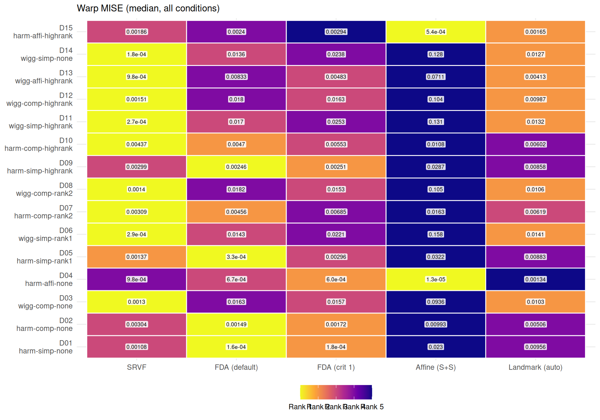
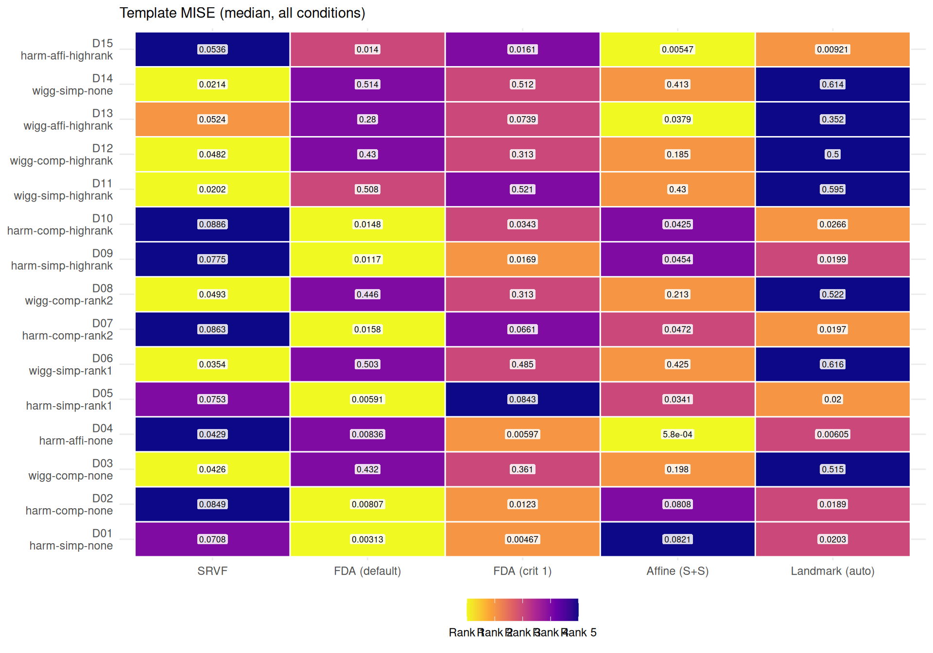
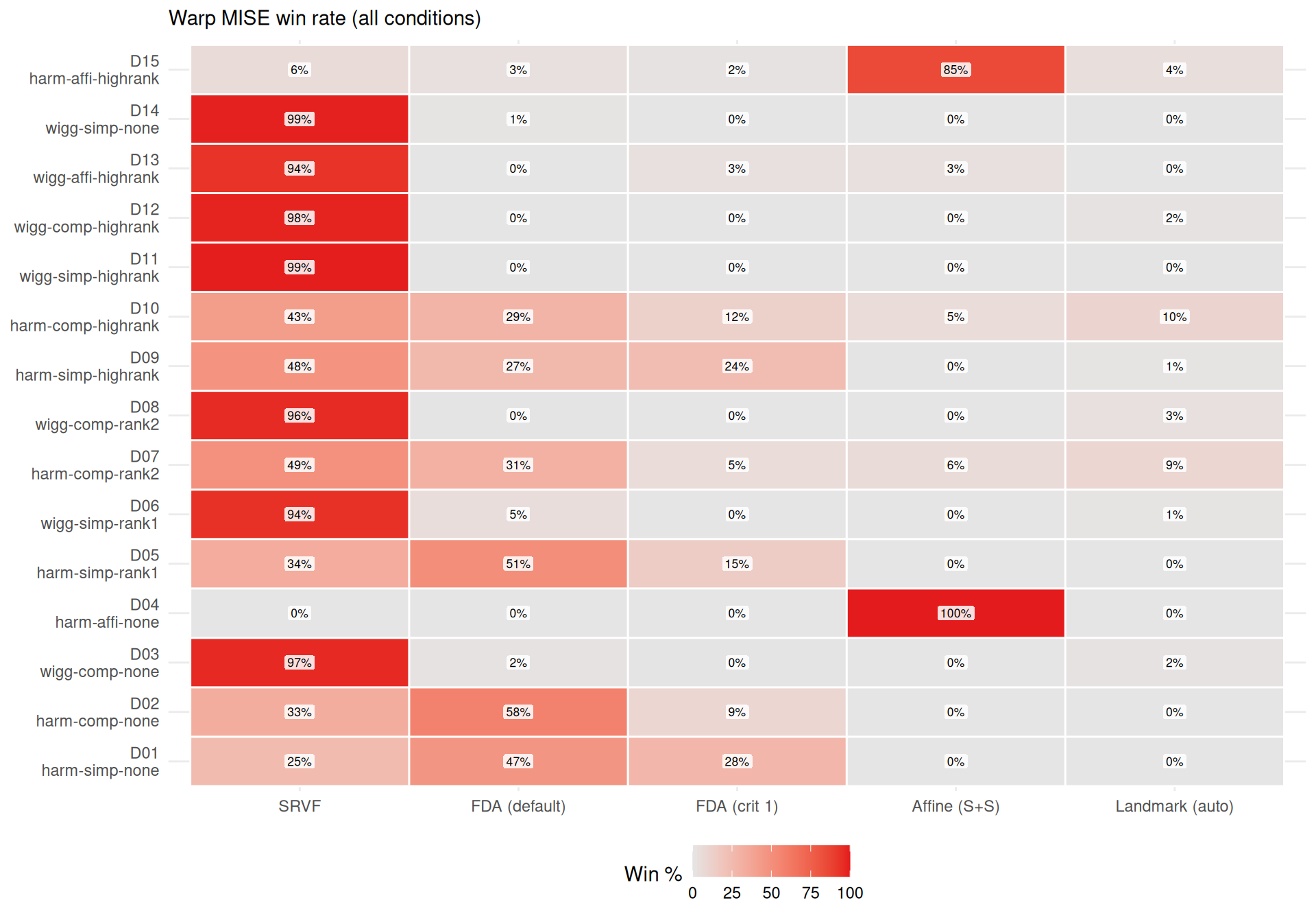
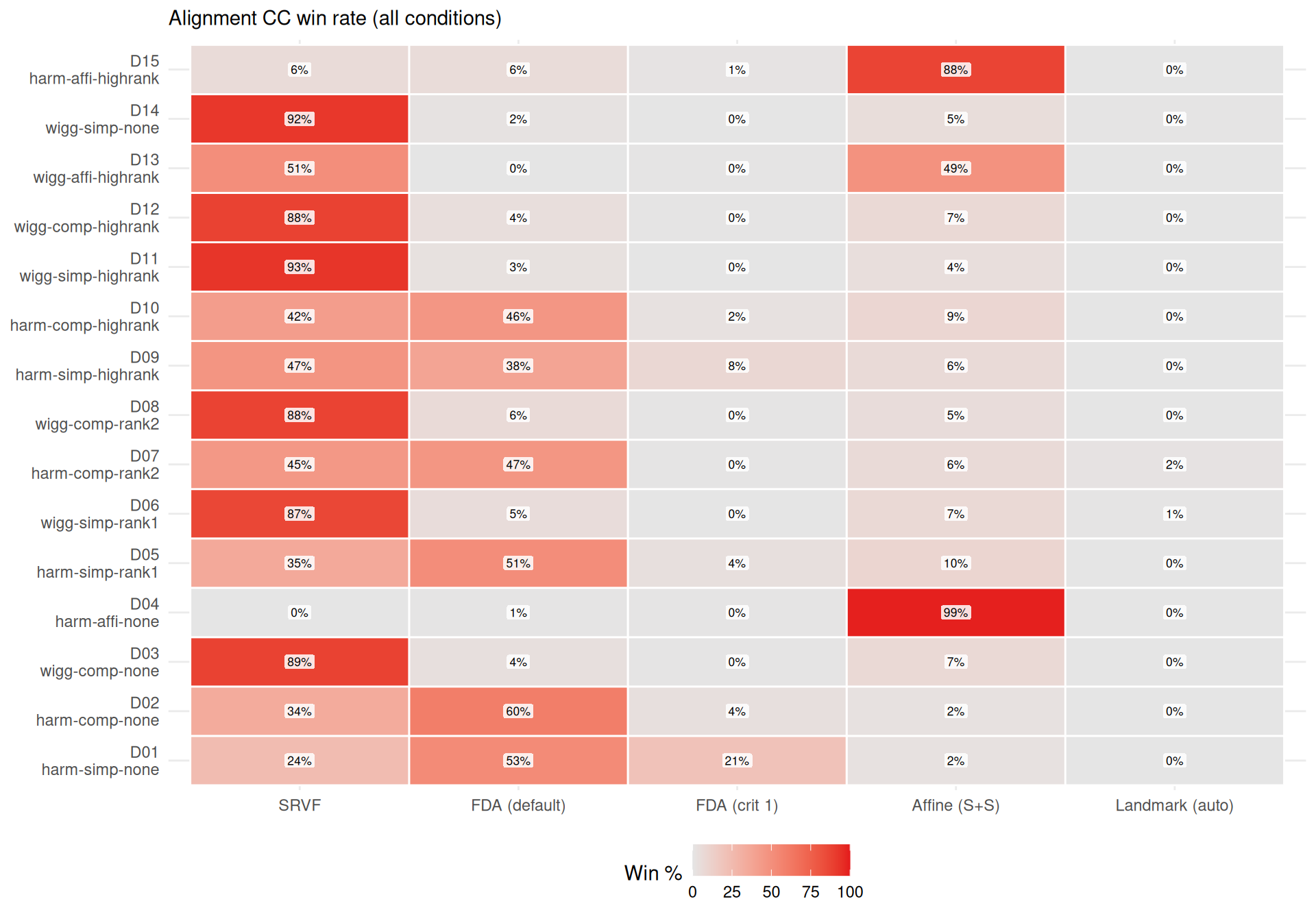
  wr <- agg_both[, .(win_pct = round(100 * mean(rank_e2 == 1), 1)), by = method][order(-win_pct)]

  # Noise sensitivity ratio (noise=0.3 / noise=0), conditioned on template
  noise_sens <- dt[
    failure == FALSE & !is.na(template_elastic_dist) & noise_sd %in% c("0", "0.3"),
    .(edist = median(template_elastic_dist)),
    by = .(method, template, noise_sd)
  ]
  wide <- dcast(noise_sens, method + template ~ noise_sd, value.var = "edist")
  setnames(wide, c("0", "0.3"), c("e0", "e03"))
  wide[, ratio := round(e03 / e0, 2)]
  # Summarize across templates (median of template-specific ratios)
  wide_pooled <- wide[, .(ratio = round(median(ratio), 1)), by = method]

  cat(sprintf(
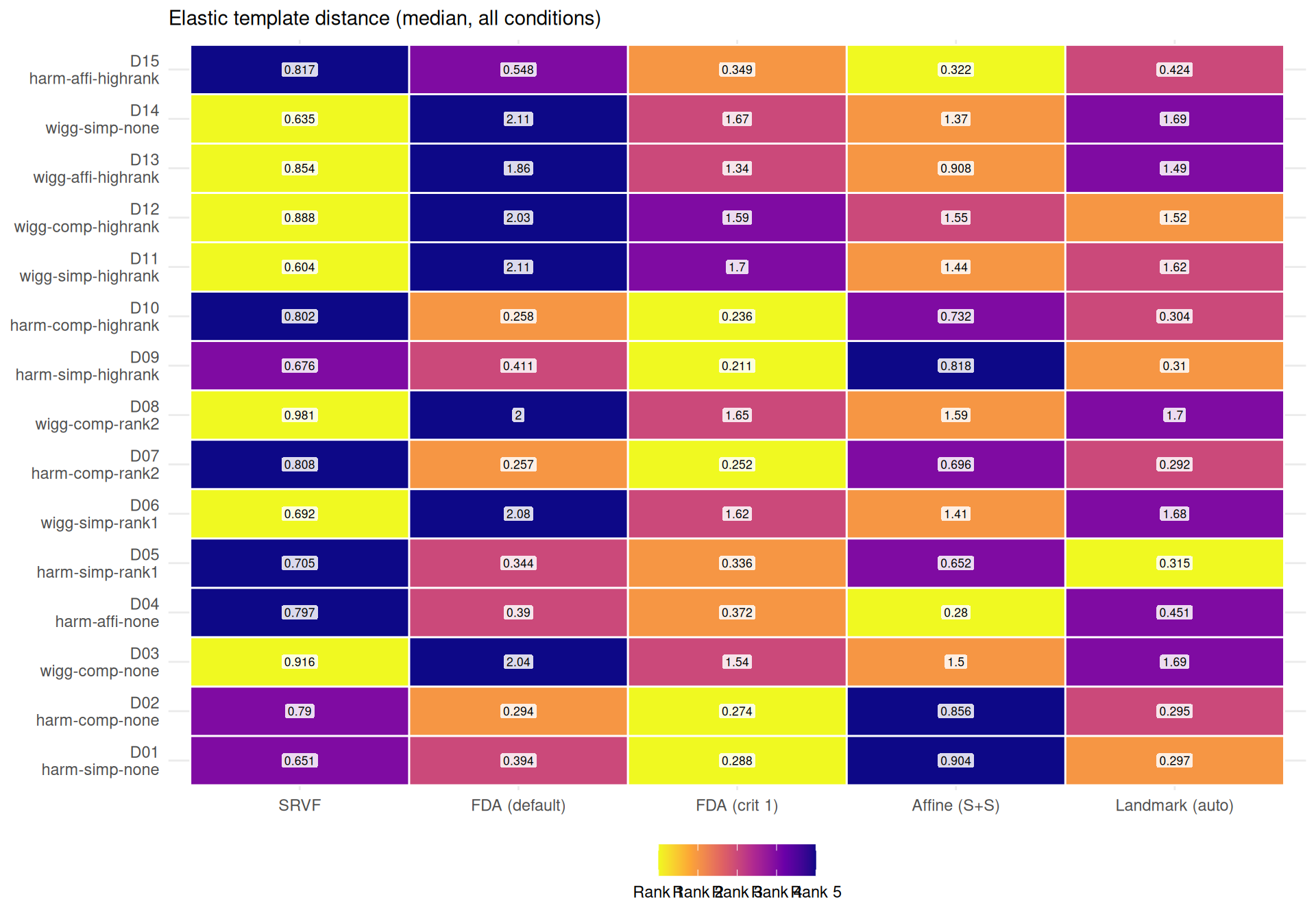
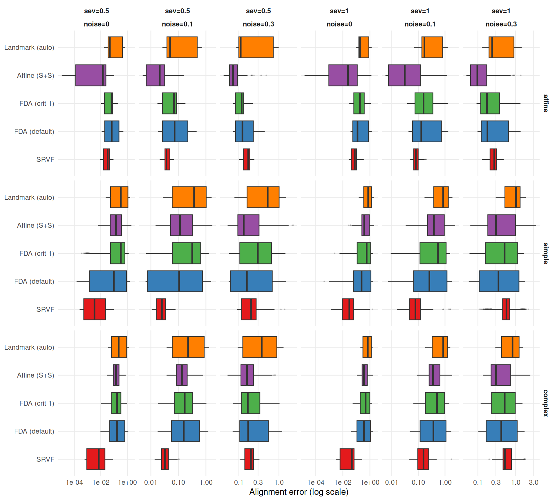
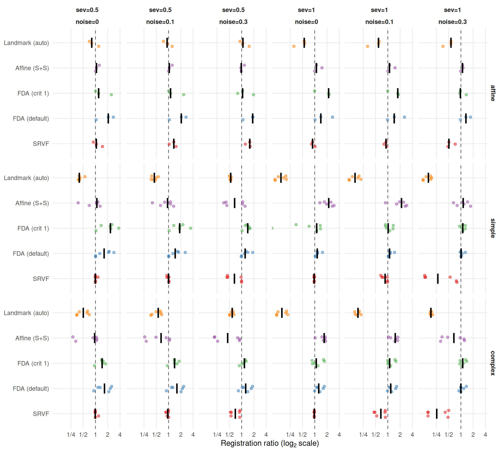
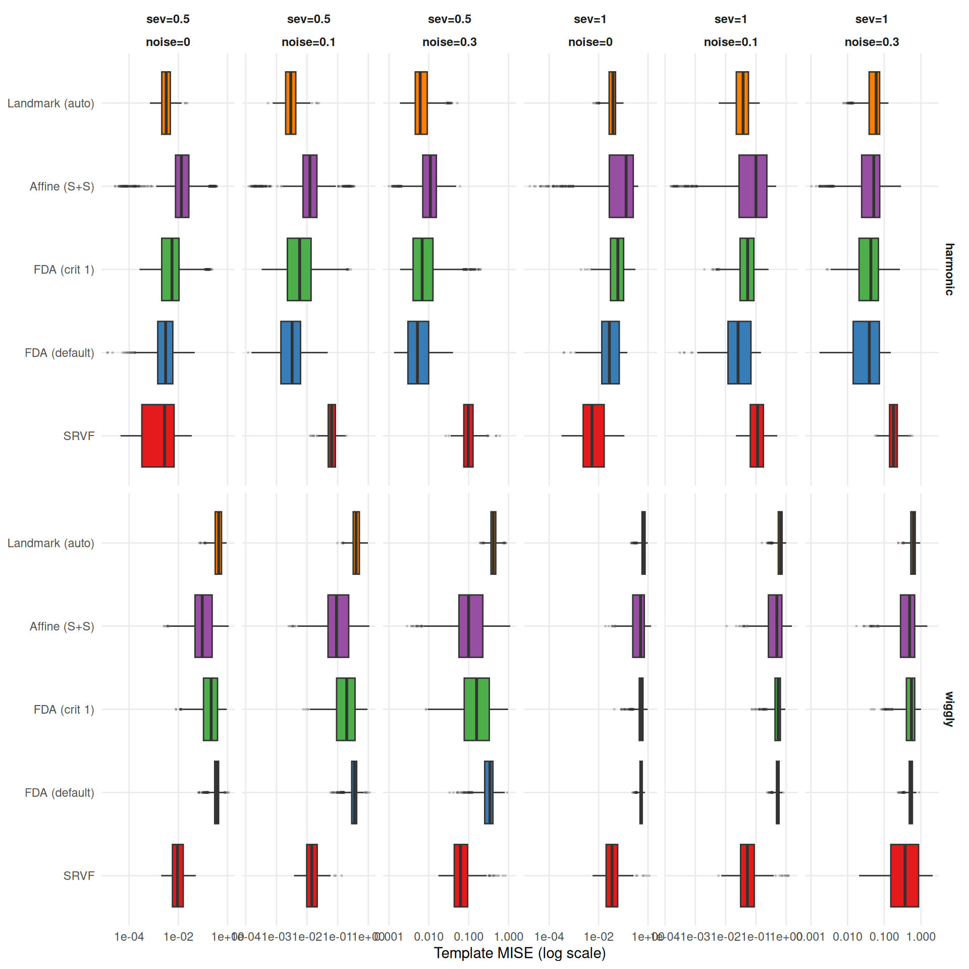
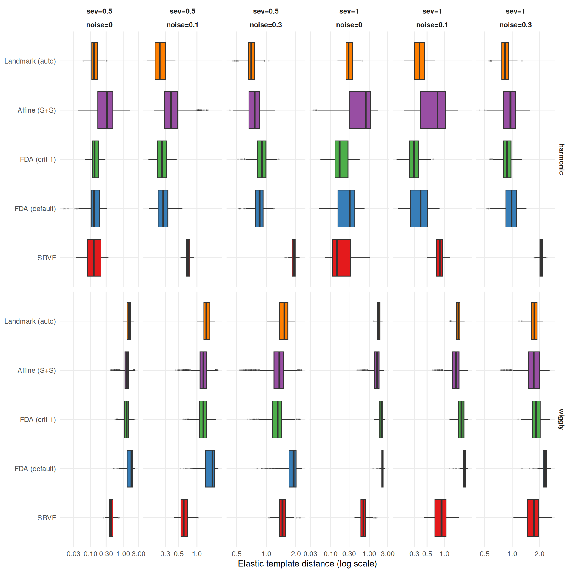
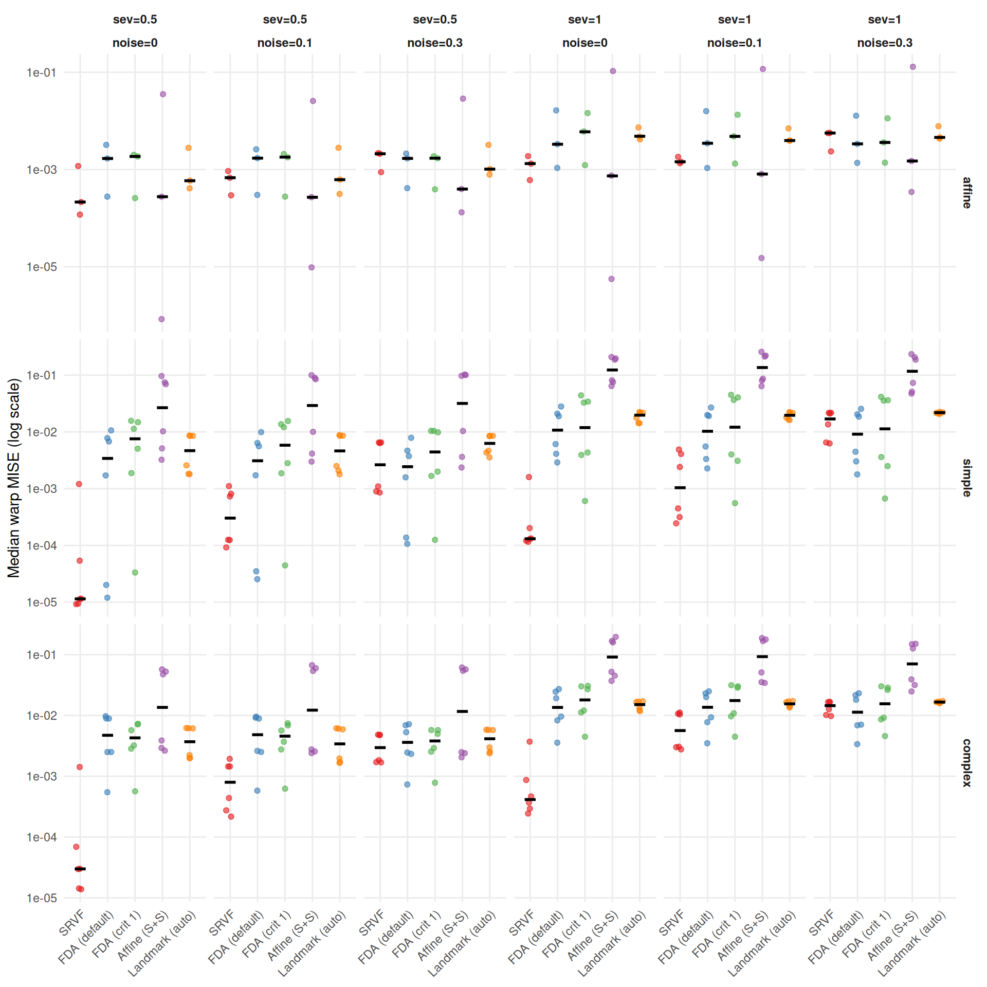
    "The two metrics agree moderately (Spearman $\\rho$ = %s across cell-level method rankings) but disagree on the best method in **%d of %d** conditions (%.0f%%). Key differences:\n\n",
    rho, n_disagree, n_total, 100 * n_disagree / n_total
  ))
  cat(sprintf(
    "- **%s** wins most often on elastic distance (%s%% of conditions), suggesting it recovers template *shape* well even when its $L^2$ MISE is mediocre (phase shifts inflate MISE but not elastic distance).\n",
    mlabs[wr$method[1]], wr$win_pct[1]
  ))
  cat(sprintf(
    "- **%s** rarely wins on elastic distance (%s%%), despite reasonable $L^2$ MISE — its templates have good pointwise fit but suboptimal shape recovery.\n",
    mlabs[wr$method[nrow(wr)]], wr$win_pct[nrow(wr)]
  ))

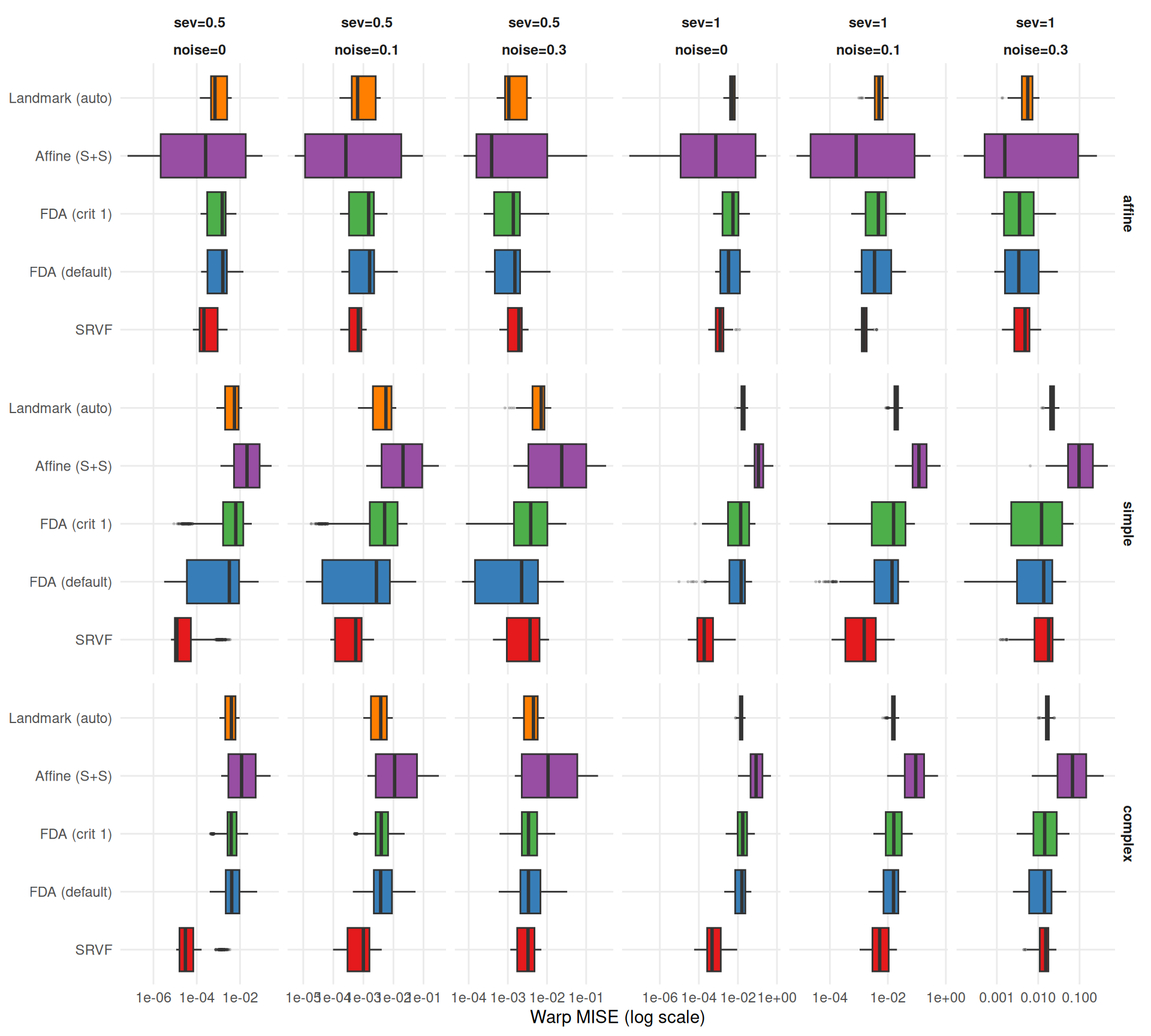
  # Noise sensitivity (template-conditioned to avoid pooling artifacts)
  srvf_ratio <- wide_pooled[method == "srvf", ratio]
  most_robust <- wide_pooled[which.min(ratio)]
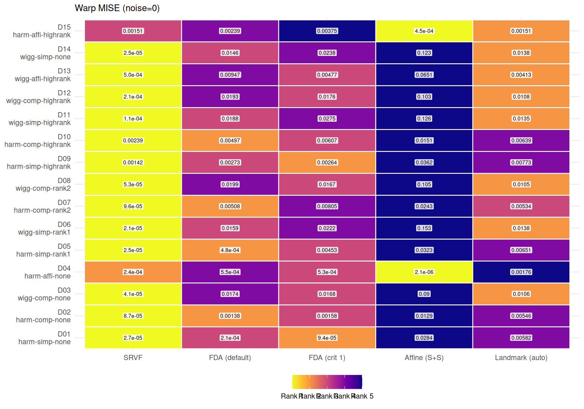
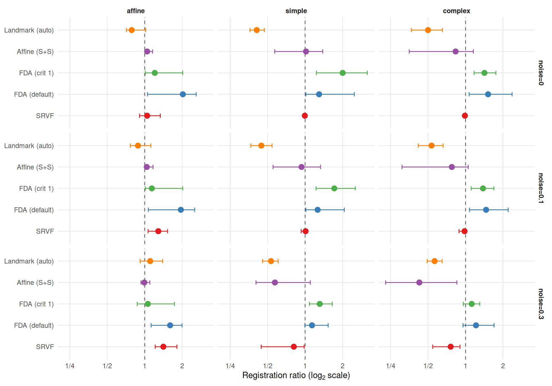
  cat(sprintf(
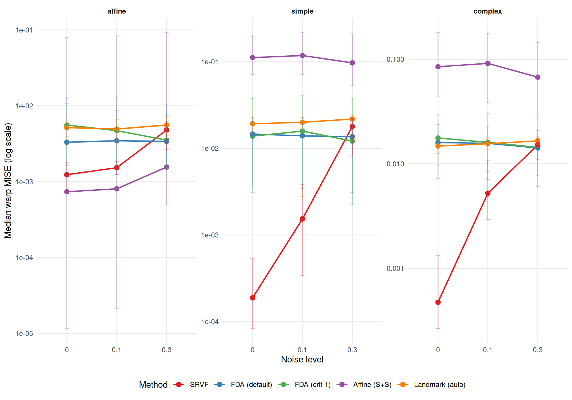
    "- **Noise sensitivity** (median ratio noise=0.3 / noise=0, conditioned on template): SRVF degrades %.1f×, while %s is most robust (%.1f×).\n",
    srvf_ratio, mlabs[most_robust$method], most_robust$ratio
  ))
  # Affine: show per-template ratios since pooling can mask heterogeneity
  affine_by_tpl <- wide[method == "affine_ss"]
  if (nrow(affine_by_tpl) > 0) {
    affine_txt <- paste(sprintf("%s: %.1f×", affine_by_tpl$template, affine_by_tpl$ratio),
      collapse = ", ")
    cat(sprintf(
      "- Affine (S+S) noise sensitivity varies by template (%s) — the pooled ratio masks heterogeneity. Elastic distance is always high (median %.2f–%.2f), indicating consistent template shape distortion.\n",
      affine_txt,
      min(noise_sens[method == "affine_ss", edist]),
      max(noise_sens[method == "affine_ss", edist])
    ))
  }
} else {
  cat("*Elastic distance not available in current results.*\n")
}

The two metrics agree moderately (Spearman \(\rho\) = 0.6 across cell-level method rankings) but disagree on the best method in 34 of 90 conditions (38%). Key differences:

SRVF wins most often on elastic distance (38.9% of conditions), suggesting it recovers template shape well even when its \(L^2\) MISE is mediocre (phase shifts inflate MISE but not elastic distance).
FDA (default) rarely wins on elastic distance (6.7%), despite reasonable \(L^2\) MISE — its templates have good pointwise fit but suboptimal shape recovery.
Noise sensitivity (median ratio noise=0.3 / noise=0, conditioned on template): SRVF degrades 8.7×, while Affine (S+S) is most robust (1.5×).
Affine (S+S) noise sensitivity varies by template (harmonic: 1.9×, wiggly: 1.1×) — the pooled ratio masks heterogeneity. Elastic distance is always high (median 0.44–1.49), indicating consistent template shape distortion.

Code

cat("\n\n")

5 Sensitivity & Variance Decomposition (Q6)

Question: Which factors most influence each metric, and how do noise and severity interact with method and DGP characteristics?

5.1 Median warp MISE across all conditions

Code

agg_q6 <- dt[failure == FALSE,
  .(mise = median(warp_mise, na.rm = TRUE)),
  by = .(dgp, method, warp_type, severity, noise_sd)]

ggplot(agg_q6, aes(x = method, y = mise, color = method)) +
  geom_jitter(width = 0.15, size = 1.5, alpha = 0.6) +
  stat_summary(fun = median, geom = "crossbar", width = 0.4,
    color = "black", linewidth = 0.4) +
  facet_grid(
    warp_type ~ severity + noise_sd,
    scales = "free_y",
    labeller = cond_labeller
  ) +
  scale_color_manual(values = mcols, labels = mlabs, guide = "none") +
  scale_x_discrete(labels = mlabs) +
  scale_y_log10() +
  labs(x = NULL, y = "Median warp MISE (log scale)") +
  theme_benchmark() +
  theme(axis.text.x = element_text(angle = 45, hjust = 1))

Median warp MISE by method across all severity × noise conditions, stratified by warp type (rows). Each dot = one DGP; crossbar = median across DGPs.

Code

# Degradation ratios — noise
ratios <- degradation_ratios(dt)
noise_rat <- ratios$noise[is.finite(noise_ratio)]
noise_rat <- merge(noise_rat, dgp_factors(), by = "dgp")

cat("**Noise × method × warp type interaction:**\n\n")

Noise × method × warp type interaction:

Code

for (wt in c("simple", "complex", "affine")) {
  cat(sprintf("*%s warps:*\n\n", wt))
  for (nl in sort(unique(as.character(noise_rat$noise_sd)))) {
    sub <- noise_rat[warp_type == wt & noise_sd == nl & severity == "0.5",
      .(ratio = median(noise_ratio, na.rm = TRUE)), by = method][order(-ratio)]
    most <- sub[1]
    least <- sub[.N]
    cat(sprintf(
      "- noise=%s: strongest degradation for %s (%.1f$\\times$), weakest for %s (%.2f$\\times$)\n",
      nl, mlabs[most$method], most$ratio, mlabs[least$method], least$ratio
    ))
  }
  cat("\n")
}

simple warps:

noise=0.1: strongest degradation for SRVF (11.7\(\times\)), weakest for FDA (default) (0.97\(\times\))
noise=0.3: strongest degradation for SRVF (106.8\(\times\)), weakest for FDA (crit 1) (0.78\(\times\))

complex warps:

noise=0.1: strongest degradation for SRVF (23.2\(\times\)), weakest for Landmark (auto) (0.92\(\times\))
noise=0.3: strongest degradation for SRVF (125.2\(\times\)), weakest for FDA (default) (0.87\(\times\))

affine warps:

noise=0.1: strongest degradation for SRVF (1.4\(\times\)), weakest for Affine (S+S) (0.97\(\times\))
noise=0.3: strongest degradation for SRVF (4.1\(\times\)), weakest for FDA (crit 1) (0.94\(\times\))

Code

# SRVF noise note
cat("SRVF operates on SRSFs (derivatives), amplifying high-frequency noise — this is the dominant noise sensitivity pattern. Study B (penalization) will test regularization.\n\n")

SRVF operates on SRSFs (derivatives), amplifying high-frequency noise — this is the dominant noise sensitivity pattern. Study B (penalization) will test regularization.

Code

# Explain ratio < 1 phenomenon
any_below_1 <- noise_rat[severity == "0.5", .(ratio = median(noise_ratio, na.rm = TRUE)), by = method][ratio < 1]
if (nrow(any_below_1) > 0) {
  cat(sprintf(
    "**Note on degradation ratios below 1**: %s show median noise ratio $< 1$ in some conditions, meaning warp MISE *decreases* with added noise. This likely reflects an implicit regularization effect — noise shrinks the cross-covariance estimates, producing smoother (less aggressive) warps that happen to be closer to the truth when the clean-data algorithm slightly over-registers. This should not be interpreted as 'noise helps registration'.\n\n",
    paste(mlabs[any_below_1$method], collapse = " and ")
  ))
}

Note on degradation ratios below 1: FDA (default) and FDA (crit 1) show median noise ratio \(< 1\) in some conditions, meaning warp MISE decreases with added noise. This likely reflects an implicit regularization effect — noise shrinks the cross-covariance estimates, producing smoother (less aggressive) warps that happen to be closer to the truth when the clean-data algorithm slightly over-registers. This should not be interpreted as ‘noise helps registration’.

Code

# Severity
sev_rat <- ratios$severity[is.finite(severity_ratio)]
sev_rat <- merge(sev_rat, dgp_factors(), by = "dgp")
sev_agg <- sev_rat[, .(ratio = median(severity_ratio, na.rm = TRUE)),
  by = .(method, warp_type)][order(warp_type, -ratio)]
cat("**Severity effect** (pooled over noise):\n\n")

Severity effect (pooled over noise):

Code

for (wt in c("simple", "complex", "affine")) {
  sub <- sev_agg[warp_type == wt]
  most <- sub[1]
  least <- sub[.N]
  cat(sprintf(
    "- *%s*: strongest for %s (%.1f$\\times$), weakest for %s (%.1f$\\times$)\n",
    wt, mlabs[most$method], most$ratio, mlabs[least$method], least$ratio
  ))
}

simple: strongest for Affine (S+S) (4.9\(\times\)), weakest for FDA (crit 1) (2.9\(\times\))
complex: strongest for SRVF (7.1\(\times\)), weakest for FDA (default) (3.1\(\times\))
affine: strongest for Landmark (auto) (5.5\(\times\)), weakest for SRVF (2.7\(\times\))

Code

cat("\n")

5.2 Method × noise interaction

The most actionable Study A finding is the interaction between method and noise level. This plot directly shows how each method’s performance changes with noise, stratified by warp type.

Code

mn_agg <- dt[failure == FALSE & severity == "1",
  .(
    mise = median(warp_mise, na.rm = TRUE),
    q25 = quantile(warp_mise, 0.25, na.rm = TRUE),
    q75 = quantile(warp_mise, 0.75, na.rm = TRUE)
  ),
  by = .(method, warp_type, noise_sd)]

ggplot(mn_agg, aes(x = noise_sd, y = mise, color = method, group = method)) +
  geom_line(linewidth = 0.8) +
  geom_point(size = 2.5) +
  geom_errorbar(aes(ymin = q25, ymax = q75), width = 0.08, alpha = 0.35) +
  facet_wrap(~ warp_type, scales = "free_y") +
  scale_color_manual(values = mcols, labels = mlabs) +
  scale_y_log10() +
  labs(x = "Noise level", y = "Median warp MISE (log scale)", color = "Method") +
  theme_benchmark()

Method × noise interaction for warp MISE (severity=1.0). Points show medians and vertical bars show IQRs. Lines connect noise levels within each method. Diverging lines indicate differential noise sensitivity.

Code

# Check for rank reversals between noise=0 and highest noise
mn_ranks <- mn_agg[, .(best = method[which.min(mise)]), by = .(warp_type, noise_sd)]
mn_wide <- dcast(mn_ranks, warp_type ~ noise_sd, value.var = "best")
highest_noise_col <- names(mn_wide)[ncol(mn_wide)]

cat("**Method × noise interaction:**\n\n")

Method × noise interaction:

Code

for (i in seq_len(nrow(mn_wide))) {
  wt <- mn_wide$warp_type[i]
  clean_best <- mlabs[mn_wide[["0"]][i]]
  noisy_best <- mlabs[mn_wide[[highest_noise_col]][i]]
  if (mn_wide[["0"]][i] == mn_wide[[highest_noise_col]][i]) {
    cat(sprintf("- **%s** warps: %s holds rank 1 from noise=0 to noise=%s.\n",
      wt, clean_best, highest_noise_col))
  } else {
    cat(sprintf("- **%s** warps: **rank reversal** — %s best at noise=0, %s best at noise=%s.\n",
      wt, clean_best, noisy_best, highest_noise_col))
  }
}

affine warps: Affine (S+S) holds rank 1 from noise=0 to noise=0.3.
simple warps: rank reversal — SRVF best at noise=0, FDA (crit 1) best at noise=0.3.
complex warps: rank reversal — SRVF best at noise=0, FDA (default) best at noise=0.3.

Code

cat("\n")

5.3 ANOVA variance decomposition

For each metric, we fit a factorial ANOVA with all main effects and 2nd-order interactions of the design factors (method, template, warp type, amplitude, severity, noise) and report \(\eta^2 = \text{SS}_\text{term} / \text{SS}_\text{total}\) for the 10 most important terms. We use Type II sums of squares (car::Anova(type = "II")) because the DGP design is not full factorial (15 of 24 cells), making Type I SS order-dependent. Type II SS tests each term after all other terms of equal or lower order, giving stable \(\eta^2\) regardless of factor ordering. Metrics that are plotted on a log scale (MISE, ratios, runtime) are log-transformed before fitting to match the analysis scale and stabilize variance.

Code

#' Compute eta-squared from Type II ANOVA for a given metric
#' Returns top-k terms by eta-squared
#' Uses car::Anova(type = "II") for stable SS in non-full-factorial design.
#' Metrics plotted on log scale are log-transformed before ANOVA.
compute_anova_eta2 <- function(dt, metric, use_log = FALSE, k = 10) {
  d <- dt[failure == FALSE & !is.na(get(metric))]
  if (use_log) {
    d <- d[get(metric) > 0]
    d[, (metric) := log(get(metric))]
  }
  for (v in c("method", "template", "warp_type", "amplitude", "severity", "noise_sd")) {
    d[[v]] <- factor(d[[v]])
  }
  fml <- as.formula(paste0(
    metric,
    " ~ (method + template + warp_type + amplitude + severity + noise_sd)^2"
  ))
  fit <- lm(fml, data = d)
  a2 <- car::Anova(fit, type = "II")
  ss_df <- data.table(
    term = rownames(a2),
    ss = a2$`Sum Sq`,
    df = a2$Df,
    f = a2$`F value`,
    p = a2$`Pr(>F)`
  )
  ss_df <- ss_df[term != "Residuals"]
  ss_total <- sum(ss_df$ss, na.rm = TRUE) + a2["Residuals", "Sum Sq"]
  ss_df[, eta2 := ss / ss_total]
  ss_df[order(-eta2)][seq_len(min(k, .N))]
}

# Metrics to analyze — with log-scale flag matching plot scales
metrics_for_anova <- list(
  list(metric = "warp_mise",                  label = "Warp MISE",                log = TRUE),
  list(metric = "alignment_error",            label = "Alignment error",           log = TRUE),
  list(metric = "template_mise",              label = "Template MISE",             log = TRUE),
  list(metric = "alignment_cc",               label = "Alignment CC",              log = FALSE),
  list(metric = "registration_ratio_median",  label = "Registration ratio",        log = TRUE),
  list(metric = "amp_variance_ratio",         label = "Amplitude variance ratio",  log = TRUE),
  list(metric = "warp_slope_ratio_median",    label = "Warp slope ratio",          log = TRUE),
  list(metric = "time_per_curve",             label = "Time per curve",            log = TRUE)
)

for (spec in metrics_for_anova) {
  metric <- spec$metric
  label <- spec$label
  use_log <- spec$log

  # Skip if metric not in data or all NA
  if (!(metric %in% names(dt))) next
  if (all(is.na(dt[[metric]]))) next

  top <- tryCatch(
    compute_anova_eta2(dt, metric, use_log = use_log),
    error = function(e) NULL
  )
  if (is.null(top) || nrow(top) == 0) next

  scale_note <- if (use_log) " (log scale)" else ""
  cat(sprintf("\n### %s%s\n\n", label, scale_note))
  top[, eta2_pct := sprintf("%.1f%%", 100 * eta2)]
  top[, stars := ifelse(is.na(p), "",
    ifelse(p < 0.001, "***",
      ifelse(p < 0.01, "**",
        ifelse(p < 0.05, "*", ""))))]
  print(knitr::kable(
    top[, .(Term = term, df, `eta^2` = eta2_pct, `F` = round(f, 1), Sig = stars)],
    caption = sprintf("Top 10 terms by eta-squared for %s%s.", label, scale_note)
  ))
  cat("\n")

  # Brief data-driven summary
  top1 <- top$term[1]
  top1_eta2 <- top$eta2[1]
  top3 <- top$term[1:min(3, nrow(top))]
  cat(sprintf(
    "The dominant source of variation is **%s** ($\\eta^2$ = %.1f%%). The top 3 terms (%s) together explain %.1f%% of total variance.\n\n",
    top1, 100 * top1_eta2,
    paste(top3, collapse = ", "),
    100 * sum(top$eta2[1:min(3, nrow(top))])
  ))
}

5.3.1 Warp MISE (log scale)

Top 10 terms by eta-squared for Warp MISE (log scale).
Term	df	eta^2	F	Sig
method	4	22.1%	13313	***
severity	1	14.8%	35744	***
method:template	4	10.8%	6519	***
template	1	7.5%	18128	***
method:noise_sd	8	7.4%	2224	***
method:warp_type	8	5.6%	1686	***
warp_type	2	4.7%	5708	***
amplitude	3	2.7%	2149	***
noise_sd	2	2.4%	2848	***
method:amplitude	12	1.0%	207	***

The dominant source of variation is method (\(\eta^2\) = 22.1%). The top 3 terms (method, severity, method:template) together explain 47.8% of total variance.

5.3.2 Alignment error (log scale)

Top 10 terms by eta-squared for Alignment error (log scale).
Term	df	eta^2	F	Sig
template	1	21.7%	52482	***
method	4	14.2%	8594	***
severity	1	9.8%	23828	***
method:noise_sd	8	7.2%	2182	***
noise_sd	2	7.2%	8725	***
method:template	4	7.1%	4301	***
method:warp_type	8	4.4%	1334	***
amplitude	3	2.6%	2064	***
warp_type	2	1.9%	2308	***
method:amplitude	12	1.3%	267	***

The dominant source of variation is template (\(\eta^2\) = 21.7%). The top 3 terms (template, method, severity) together explain 45.7% of total variance.

5.3.3 Template MISE (log scale)

Top 10 terms by eta-squared for Template MISE (log scale).
Term	df	eta^2	F	Sig
template	1	36.7%	88025	***
severity	1	12.9%	30893	***
method:template	4	10.9%	6533	***
method:noise_sd	8	6.6%	1980	***
method:warp_type	8	4.7%	1403	***
warp_type	2	2.1%	2518	***
noise_sd	2	2.0%	2380	***
method	4	1.4%	827	***
amplitude	3	1.0%	813	***
template:severity	1	0.8%	2035	***

The dominant source of variation is template (\(\eta^2\) = 36.7%). The top 3 terms (template, severity, method:template) together explain 60.5% of total variance.

5.3.4 Alignment CC

Top 10 terms by eta-squared for Alignment CC.
Term	df	eta^2	F	Sig
template	1	37.1%	84516	***
method	4	11.6%	6598	***
method:template	4	11.1%	6340	***
severity	1	9.3%	21194	***
template:severity	1	3.4%	7823	***
warp_type	2	2.0%	2288	***
method:noise_sd	8	1.6%	460	***
template:warp_type	2	1.5%	1681	***
noise_sd	2	0.9%	1026	***
method:warp_type	8	0.6%	182	***

The dominant source of variation is template (\(\eta^2\) = 37.1%). The top 3 terms (template, method, method:template) together explain 59.8% of total variance.

5.3.5 Registration ratio (log scale)

Top 10 terms by eta-squared for Registration ratio (log scale).
Term	df	eta^2	F	Sig
method	4	41.7%	17197	***
method:severity	4	10.8%	4448	***
severity	1	2.9%	4841	***
method:warp_type	8	2.8%	577	***
warp_type	2	2.6%	2173	***
method:noise_sd	8	2.5%	517	***
noise_sd	2	2.3%	1922	***
template	1	2.1%	3414	***
method:template	4	1.8%	731	***
amplitude	3	0.7%	362	***

The dominant source of variation is method (\(\eta^2\) = 41.7%). The top 3 terms (method, method:severity, severity) together explain 55.4% of total variance.

5.3.6 Amplitude variance ratio (log scale)

Top 10 terms by eta-squared for Amplitude variance ratio (log scale).
Term	df	eta^2	F	Sig
template	1	27.5%	59272	***
method	4	21.6%	11625	***
method:template	4	15.3%	8247	***
noise_sd	2	8.5%	9157	***
severity	1	7.1%	15262	***
method:noise_sd	8	2.7%	736	***
warp_type	2	1.5%	1621	***
template:noise_sd	2	1.5%	1594	***
template:warp_type	2	0.7%	725	***
method:warp_type	8	0.4%	121	***

The dominant source of variation is template (\(\eta^2\) = 27.5%). The top 3 terms (template, method, method:template) together explain 64.5% of total variance.

5.3.7 Warp slope ratio (log scale)

Top 10 terms by eta-squared for Warp slope ratio (log scale).
Term	df	eta^2	F	Sig
method	4	97.8%	481905.0	***
severity	1	0.1%	1321.9	***
warp_type	1	0.1%	1086.7	***
method:template	4	0.1%	262.3	***
method:amplitude	12	0.0%	54.3	***
method:warp_type	4	0.0%	155.7	***
method:noise_sd	8	0.0%	67.9	***
method:severity	4	0.0%	89.0	***
warp_type:noise_sd	2	0.0%	130.2	***
template:severity	1	0.0%	251.7	***

The dominant source of variation is method (\(\eta^2\) = 97.8%). The top 3 terms (method, severity, warp_type) together explain 97.9% of total variance.

5.3.8 Time per curve (log scale)

Top 10 terms by eta-squared for Time per curve (log scale).
Term	df	eta^2	F	Sig
method	4	95.6%	303190	***
noise_sd	2	0.1%	866	***
method:warp_type	8	0.1%	216	***
method:amplitude	12	0.1%	129	***
method:noise_sd	8	0.1%	178	***
method:template	4	0.1%	287	***
method:severity	4	0.1%	285	***
severity:noise_sd	2	0.1%	459	***
template	1	0.0%	399	***
template:noise_sd	2	0.0%	172	***

The dominant source of variation is method (\(\eta^2\) = 95.6%). The top 3 terms (method, noise_sd, method:warp_type) together explain 95.8% of total variance.

6 Practical (Q7)

6.1 Runtime

Code

ggplot(
  dt[failure == FALSE],
  aes(y = method, x = time_per_curve, fill = method)
) +
  geom_boxplot(outlier.size = 0.3, outlier.alpha = 0.2) +
  scale_fill_manual(values = mcols, labels = mlabs, guide = "none") +
  scale_y_discrete(labels = mlabs) +
  scale_x_log10() +
  labs(y = NULL, x = "Time per curve (seconds, log scale)") +
  theme_benchmark()

Distribution of time per curve (seconds) by method across all conditions. Log10 scale. Boxplots show all non-failed runs.

Code

time_tbl <- dt[failure == FALSE, .(
  median = round(median(time_per_curve, na.rm = TRUE), 3),
  q25 = round(quantile(time_per_curve, 0.25, na.rm = TRUE), 3),
  q75 = round(quantile(time_per_curve, 0.75, na.rm = TRUE), 3)
), by = method][order(-median)]

knitr::kable(time_tbl,
  col.names = c("Method", "Median (s)", "Q25 (s)", "Q75 (s)"),
  caption = "Time per curve (seconds) across all conditions."
)

Time per curve (seconds) across all conditions.
Method	Median (s)	Q25 (s)	Q75 (s)
fda_crit1	0.200	0.165	0.264
srvf	0.180	0.179	0.181
fda_default	0.118	0.105	0.162
affine_ss	0.094	0.070	0.127
landmark_auto	0.003	0.003	0.004

Code

rt <- dt[failure == FALSE, .(
  med = median(time_per_curve, na.rm = TRUE)
), by = method][order(-med)]

cat("**Runtime findings:**\n\n")

Runtime findings:

Code

for (i in seq_len(nrow(rt))) {
  cat(sprintf("- **%s**: %.3f s/curve\n", mlabs[rt$method[i]], rt$med[i]))
}

FDA (crit 1): 0.200 s/curve
SRVF: 0.180 s/curve
FDA (default): 0.118 s/curve
Affine (S+S): 0.094 s/curve
Landmark (auto): 0.003 s/curve

Code

fastest <- rt[.N]
slowest <- rt[1]
ratio <- slowest$med / fastest$med
cat(sprintf(
  "\n%s is %.0f$\\times$ slower than %s (the fastest).\n\n",
  mlabs[slowest$method], ratio, mlabs[fastest$method]
))

FDA (crit 1) is 58\(\times\) slower than Landmark (auto) (the fastest).

6.2 Failures

Code

fail_tbl <- failure_summary(dt)
fail_tbl[, rate := round(rate, 3)]
knitr::kable(
  fail_tbl[order(method, warp_type)],
  col.names = c("Method", "Warp type", "N total", "N failed", "Rate"),
  caption = "Failure rates by method and warp type."
)

Failure rates by method and warp type.
Method	Warp type	N total	N failed	Rate
srvf	affine	1800	0	0.000
srvf	simple	3600	0	0.000
srvf	complex	3600	0	0.000
fda_default	affine	1800	0	0.000
fda_default	simple	3600	0	0.000
fda_default	complex	3600	0	0.000
fda_crit1	affine	1800	0	0.000
fda_crit1	simple	3600	0	0.000
fda_crit1	complex	3600	0	0.000
affine_ss	affine	1800	0	0.000
affine_ss	simple	3600	0	0.000
affine_ss	complex	3600	0	0.000
landmark_auto	affine	1800	0	0.000
landmark_auto	simple	3600	8	0.002
landmark_auto	complex	3600	2	0.001

Code

err <- dt[failure == TRUE & nchar(error_msg) > 0]
err[, error_class := fcase(
  grepl("monotonic", error_msg), "Non-monotonic warp",
  grepl("duplicated values", error_msg), "Duplicated arg values in warped curves",
  grepl("computationally singular", error_msg), "Singular linear system",
  grepl("missing value where TRUE/FALSE", error_msg), "NA in logical comparison",
  default = "Other"
)]

cat("**Error analysis:**\n\n")

Error analysis:

Code

cat(sprintf("Total failures: %d out of %d runs (%.2f%%).\n\n",
  sum(dt$failure), nrow(dt), 100 * mean(dt$failure)))

Total failures: 10 out of 45000 runs (0.02%).

Code

if (sum(dt$failure) == 0) {
  cat("No failures — all runs completed successfully.\n\n")
} else {
  # Failures by method
  fail_by_method <- dt[failure == TRUE, .N, by = method][order(-N)]
  cat("Failures by method:\n\n")
  for (i in seq_len(nrow(fail_by_method))) {
    m <- fail_by_method$method[i]
    n <- fail_by_method$N[i]
    n_total <- dt[method == m, .N]
    cat(sprintf("- **%s**: %d failures (%.2f%%)\n",
      mlabs[m], n, 100 * n / n_total))
  }
  cat("\n")

  # Error classes
  if (nrow(err) > 0) {
    err_summary <- err[, .N, by = error_class][order(-N)]
    cat("Error types:\n\n")
    for (i in seq_len(nrow(err_summary))) {
      cat(sprintf("- **%s** (%d cases)\n",
        err_summary$error_class[i], err_summary$N[i]))
    }
    cat("\n")

    # DGP concentration
    fail_by_dgp <- err[, .N, by = dgp][order(-N)]
    if (nrow(fail_by_dgp) <= 5) {
      cat(sprintf("Failures concentrated in %d DGP(s): %s.\n\n",
        nrow(fail_by_dgp),
        paste(sprintf("%s (%d)", fail_by_dgp$dgp, fail_by_dgp$N),
          collapse = ", ")))
    }
  }
}

Failures by method:

Landmark (auto): 10 failures (0.11%)

Error types:

Non-monotonic warp (10 cases)

Failures concentrated in 4 DGP(s): D09 (5), D01 (3), D02 (1), D10 (1).

7 Data Completeness

Code

comp <- dt[, .N, by = .(dgp, method)]
comp_wide <- dcast(comp, dgp ~ method, value.var = "N")
knitr::kable(comp_wide,
  caption = "Number of runs per DGP x method (target: 600 = 2 severity x 3 noise x 100 reps). Missing cells indicate batches that did not complete on the cluster."
)

Number of runs per DGP x method (target: 600 = 2 severity x 3 noise x 100 reps). Missing cells indicate batches that did not complete on the cluster.
dgp	srvf	fda_default	fda_crit1	affine_ss	landmark_auto
D01	600	600	600	600	600
D02	600	600	600	600	600
D03	600	600	600	600	600
D04	600	600	600	600	600
D05	600	600	600	600	600
D06	600	600	600	600	600
D07	600	600	600	600	600
D08	600	600	600	600	600
D09	600	600	600	600	600
D10	600	600	600	600	600
D11	600	600	600	600	600
D12	600	600	600	600	600
D13	600	600	600	600	600
D14	600	600	600	600	600
D15	600	600	600	600	600

Code

expected <- CJ(
  dgp = levels(dt$dgp),
  method = levels(dt$method)
)
actual <- unique(dt[, .(dgp, method)])
missing <- expected[!actual, on = .(dgp, method)]
if (nrow(missing) > 0) {
  cat("**Missing DGP x method combinations** (", nrow(missing),
    " batches still running on LRZ):\n\n", sep = "")
  for (i in seq_len(nrow(missing))) {
    cat(sprintf("- %s / %s\n", missing$dgp[i], missing$method[i]))
  }
} else {
  cat("All DGP x method combinations present.\n")
}

All DGP x method combinations present.

8 Summary

Code

cat("## Key findings\n\n")

8.1 Key findings

Code

# 1. Best method for warp recovery
best_by_wt <- dt[failure == FALSE,
  .(mise = median(warp_mise, na.rm = TRUE)),
  by = .(method, warp_type)
][, .(best = method[which.min(mise)]), by = warp_type]
best_overall <- dt[failure == FALSE & warp_type != "affine",
  .(mise = median(warp_mise, na.rm = TRUE)),
  by = method][which.min(mise), method]
# Check: does it win on every DGP?
per_dgp <- dt[failure == FALSE & warp_type != "affine",
  .(mise = median(warp_mise, na.rm = TRUE)),
  by = .(dgp, method)
][, .(best = method[which.min(mise)]), by = dgp]
n_wins <- sum(per_dgp$best == best_overall)
n_dgps_dp <- nrow(per_dgp)

# Check if this holds on both templates
per_tpl <- dt[failure == FALSE & warp_type != "affine",
  .(mise = median(warp_mise, na.rm = TRUE)),
  by = .(method, template)
][, .(best = method[which.min(mise)]), by = template]
same_on_both <- length(unique(per_tpl$best)) == 1

if (same_on_both) {
  cat(sprintf(
    "1. **%s is the best general-purpose method** for warp recovery on domain-preserving warps (simple + complex), ranking first on %d of %d DGPs. This holds for both harmonic and wiggly templates when pooling over noise levels. However, the method:template and method:noise interactions are substantial (@sec-method-template, @sec-method-noise) — rankings can shift in specific template/noise combinations.\n\n",
    mlabs[best_overall], n_wins, n_dgps_dp
  ))
} else {
  h_best <- mlabs[per_tpl[template == "harmonic", best]]
  w_best <- mlabs[per_tpl[template == "wiggly", best]]
  cat(sprintf(
    "1. **No single best method**: %s is best on wiggly templates, but %s is best on harmonic templates (when pooling over noise). The method:template interaction (@sec-method-template) makes global 'best method' claims misleading. %s achieves the lowest *pooled* median and ranks first on %d of %d DGPs, but this reflects effect sizes within templates, not a uniform advantage.\n\n",
    w_best, h_best, mlabs[best_overall], n_wins, n_dgps_dp
  ))
}

No single best method: SRVF is best on wiggly templates, but FDA (default) is best on harmonic templates (when pooling over noise). The method:template interaction (Section 3.5) makes global ‘best method’ claims misleading. SRVF achieves the lowest pooled median and ranks first on 8 of 12 DGPs, but this reflects effect sizes within templates, not a uniform advantage.

Code

# 2. Amplitude degradation
best_highrank_sum <- dt[failure == FALSE & amplitude == "highrank",
  .(mise = median(warp_mise, na.rm = TRUE)),
  by = method][which.min(mise), method]
best_none_sum <- dt[failure == FALSE & amplitude == "none",
  .(mise = median(warp_mise, na.rm = TRUE)),
  by = method][which.min(mise), method]
cat(sprintf(
  "2. **Amplitude variation degrades warp recovery for most methods**, but the pattern is not universal (see @sec-q2 for per-ladder details). %s retains the lowest absolute MISE under high-rank amplitude.\n\n",
  mlabs[best_highrank_sum]
))

Amplitude variation degrades warp recovery for most methods, but the pattern is not universal (see Section 3.2 for per-ladder details). SRVF retains the lowest absolute MISE under high-rank amplitude.

Code

# 3. Affine DGPs
affine_best <- best_by_wt[warp_type == "affine", best]
affine_ranks <- dt[failure == FALSE & warp_type == "affine",
  .(mise = median(warp_mise, na.rm = TRUE)),
  by = method][order(mise)]
# Check if affine wins uniformly across conditions
affine_cond <- dt[failure == FALSE & warp_type == "affine",
  .(mise = median(warp_mise, na.rm = TRUE)),
  by = .(method, severity, noise_sd)
][, .(best = method[which.min(mise)]), by = .(severity, noise_sd)]
n_affine_wins <- sum(affine_cond$best == "affine_ss")
n_affine_conds <- nrow(affine_cond)

if (affine_best == "affine_ss") {
  ratio_2nd <- affine_ranks$mise[2] / affine_ranks$mise[1]
  if (n_affine_wins == n_affine_conds) {
    cat(sprintf(
      "3. **Affine (S+S) performs as expected on affine DGPs** — it achieves the lowest MISE across all %d conditions (%.1f$\\times$ lower than %s pooled). See @sec-affine-note.\n\n",
      n_affine_conds, ratio_2nd, mlabs[affine_ranks$method[2]]
    ))
  } else {
    cat(sprintf(
      "3. **Affine (S+S) wins on affine DGPs overall** (%.1f$\\times$ lower MISE than %s pooled), but not uniformly — it ranks first in %d of %d severity/noise conditions. See @sec-affine-note.\n\n",
      ratio_2nd, mlabs[affine_ranks$method[2]], n_affine_wins, n_affine_conds
    ))
  }
} else {
  cat(sprintf(
    "3. **The affine method underperforms on affine DGPs** despite being well-specified — %s achieves lower MISE (see @sec-affine-note).\n\n",
    mlabs[affine_best]
  ))
}

Affine (S+S) wins on affine DGPs overall (2.4\(\times\) lower MISE than SRVF pooled), but not uniformly — it ranks first in 5 of 6 severity/noise conditions. See Section 3.3.1.

Code

# 4. Failure rates
fail_rates <- dt[, .(rate = 100 * mean(failure)), by = method][order(-rate)]
overall_fail <- 100 * mean(dt$failure)
if (overall_fail < 0.1) {
  cat(sprintf(
    "4. **Near-zero failure rate** (%.2f%% overall). %s has the highest rate at %.2f%%. See @sec-failures for details.\n\n",
    overall_fail, mlabs[fail_rates$method[1]], fail_rates$rate[1]
  ))
} else {
  top2 <- fail_rates[1:min(2, .N)]
  cat(sprintf(
    "4. **Failure rates**: %s (%.1f%%) and %s (%.1f%%) have the highest failure rates. See @sec-failures for error analysis.\n\n",
    mlabs[top2$method[1]], top2$rate[1],
    mlabs[top2$method[min(2, nrow(top2))]], top2$rate[min(2, nrow(top2))]
  ))
}

Near-zero failure rate (0.02% overall). Landmark (auto) has the highest rate at 0.11%. See Section 6.2 for details.

Code

# 5. Noise/severity sensitivity
# Recompute here to avoid dependency on chunk-local variables
ratios_sum <- degradation_ratios(dt)
noise_sum <- ratios_sum$noise[
  severity == "0.5" & is.finite(noise_ratio),
  .(ratio = median(noise_ratio, na.rm = TRUE)),
  by = .(method, noise_sd)
][order(noise_sd, -ratio)]
sev_sum <- ratios_sum$severity[
  noise_sd == "0" & is.finite(severity_ratio),
  .(ratio = median(severity_ratio, na.rm = TRUE)),
  by = method
][order(-ratio)]
# Use highest noise level for the summary
highest_noise <- max(as.numeric(as.character(noise_sum$noise_sd)))
noise_worst_hn <- noise_sum[noise_sd == as.character(highest_noise)][which.max(ratio)]
noise_best_hn <- noise_sum[noise_sd == as.character(highest_noise)][which.min(ratio)]
sev_worst <- sev_sum[1]
noise_robust_txt <- if (noise_best_hn$ratio < 1) {
  sprintf("%s appears most robust (%.1f$\\times$, but ratios $<$ 1 likely reflect regularization artifacts, not genuine improvement from noise)",
    mlabs[noise_best_hn$method], noise_best_hn$ratio)
} else {
  sprintf("%s is most robust (%.1f$\\times$)", mlabs[noise_best_hn$method], noise_best_hn$ratio)
}
cat(sprintf(
  "5. **Noise sensitivity varies sharply**: at noise=%.1f, %s is most noise-sensitive (%.1f$\\times$ degradation ratio) and %s. At noise=0, severity hits %s hardest (%.1f$\\times$ degradation from sev=0.5 to 1.0). See @sec-sensitivity.\n\n",
  highest_noise,
  mlabs[noise_worst_hn$method], noise_worst_hn$ratio,
  noise_robust_txt,
  mlabs[sev_worst$method], sev_worst$ratio
))

Noise sensitivity varies sharply: at noise=0.3, SRVF is most noise-sensitive (97.4\(\times\) degradation ratio) and FDA (crit 1) appears most robust (0.9\(\times\), but ratios \(<\) 1 likely reflect regularization artifacts, not genuine improvement from noise). At noise=0, severity hits SRVF hardest (9.8\(\times\) degradation from sev=0.5 to 1.0). See Section 5.

Code

# 6. Landmark
lm_rank <- dt[failure == FALSE,
  .(mise = median(warp_mise, na.rm = TRUE)),
  by = .(dgp, method)
][, rank := rank(mise), by = dgp
][method == "landmark_auto", .(mean_rank = mean(rank))]
lm_fail <- fail_rates[method == "landmark_auto", rate]
cat(sprintf(
  "6. **Landmark (auto) is competitive** (mean rank %.1f across DGPs) with near-zero failure rate (%.1f%%) and fast runtime. Its weakness is under-registration (registration ratio well below 1) and variability when landmark detection is unreliable.\n\n",
  lm_rank$mean_rank, lm_fail
))

Landmark (auto) is competitive (mean rank 2.9 across DGPs) with near-zero failure rate (0.1%) and fast runtime. Its weakness is under-registration (registration ratio well below 1) and variability when landmark detection is unreliable.

Code

# 7. AVR
avr_summary <- dt[amplitude != "none" & failure == FALSE & !is.na(amp_variance_ratio),
  .(avr = median(amp_variance_ratio, na.rm = TRUE)), by = method]
overreg_methods <- avr_summary[avr < 0.9, method]
cat("7. **Phase-amplitude separation varies by method**: ")

Phase-amplitude separation varies by method:

Code

if (length(overreg_methods) > 0) {
  cat(sprintf(
    "%s show median AVR < 1, suggesting over-registration that absorbs amplitude into phase. ",
    paste(mlabs[overreg_methods], collapse = " and ")
  ))
}
underreg_methods <- avr_summary[avr > 1.1, method]
if (length(underreg_methods) > 0) {
  cat(sprintf(
    "%s show AVR > 1 (under-registration or template bias inflating residuals). ",
    paste(mlabs[underreg_methods], collapse = " and ")
  ))
}

Affine (S+S) and FDA (crit 1) and FDA (default) and Landmark (auto) and SRVF show AVR > 1 (under-registration or template bias inflating residuals).

Code

near_one <- avr_summary[avr >= 0.9 & avr <= 1.1, method]
if (length(near_one) > 0) {
  cat(sprintf(
    "%s show near-calibrated AVR. ",
    paste(mlabs[near_one], collapse = " and ")
  ))
}
cat("Note that AVR > 1 can reflect either residual phase variation or template estimation error — these effects are confounded.\n\n")

Note that AVR > 1 can reflect either residual phase variation or template estimation error — these effects are confounded.

Code

warp_med <- dt[failure == FALSE,
  .(warp_mise = round(median(warp_mise, na.rm = TRUE), 4)),
  by = method]
tpl_med <- dt[failure == FALSE,
  .(template_mise = round(median(template_mise, na.rm = TRUE), 4)),
  by = method]
rr_med <- dt[
  failure == FALSE & !is.na(registration_ratio_median),
  .(reg_ratio = round(median(registration_ratio_median, na.rm = TRUE), 2)),
  by = method
]
runtime <- dt[failure == FALSE,
  .(time_s = round(median(time_per_curve, na.rm = TRUE), 3)),
  by = method]
fail_rate <- dt[, .(fail_pct = round(100 * mean(failure), 2)), by = method]

summary_parts <- list(warp_med, tpl_med, rr_med, runtime, fail_rate)

# Add elastic distance if available
if ("template_elastic_dist" %in% names(dt)) {
  elastic_med <- dt[failure == FALSE & !is.na(template_elastic_dist),
    .(elastic_dist = round(median(template_elastic_dist, na.rm = TRUE), 4)),
    by = method]
  summary_parts <- c(summary_parts[1:2], list(elastic_med), summary_parts[3:5])
}

summary_dt <- Reduce(function(a, b) merge(a, b, by = "method"), summary_parts)

col_names <- c("Method", "Warp MISE", "Template MISE")
if ("template_elastic_dist" %in% names(dt)) col_names <- c(col_names, "Elastic dist.")
col_names <- c(col_names, "Reg. ratio", "Time/curve (s)", "Failure %")

knitr::kable(
  summary_dt[order(method)],
  col.names = col_names,
  caption = "Summary per method (medians pooled across all conditions). Pooled medians hide strong method × template and method × noise interactions — see conditional analyses above. Reg. ratio: 1 = perfectly calibrated. Time/curve: median seconds."
)

Summary per method (medians pooled across all conditions). Pooled medians hide strong method × template and method × noise interactions — see conditional analyses above. Reg. ratio: 1 = perfectly calibrated. Time/curve: median seconds.
Method	Warp MISE	Template MISE	Elastic dist.	Reg. ratio	Time/curve (s)	Failure %
srvf	0.001	0.052	0.764	0.95	0.180	0.00
fda_default	0.005	0.084	1.015	1.20	0.118	0.00
fda_crit1	0.005	0.084	0.944	1.25	0.200	0.00
affine_ss	0.046	0.080	1.048	1.04	0.094	0.00
landmark_auto	0.008	0.075	0.880	0.37	0.003	0.11

Session Info

Code

sessionInfo()

R version 4.5.2 (2025-10-31)
Platform: x86_64-pc-linux-gnu
Running under: Linux Mint 22.1

Matrix products: default
BLAS:   /usr/lib/x86_64-linux-gnu/blas/libblas.so.3.12.0 
LAPACK: /usr/lib/x86_64-linux-gnu/lapack/liblapack.so.3.12.0  LAPACK version 3.12.0

locale:
 [1] LC_CTYPE=en_US.UTF-8       LC_NUMERIC=C              
 [3] LC_TIME=en_US.UTF-8        LC_COLLATE=en_US.UTF-8    
 [5] LC_MONETARY=de_DE.UTF-8    LC_MESSAGES=en_US.UTF-8   
 [7] LC_PAPER=de_DE.UTF-8       LC_NAME=C                 
 [9] LC_ADDRESS=C               LC_TELEPHONE=C            
[11] LC_MEASUREMENT=de_DE.UTF-8 LC_IDENTIFICATION=C       

time zone: Europe/Berlin
tzcode source: system (glibc)

attached base packages:
[1] stats     graphics  grDevices utils     datasets  methods   base     

other attached packages:
[1] tf_0.4.0          car_3.1-3         carData_3.0-5     patchwork_1.3.2  
[5] data.table_1.17.8 ggplot2_4.0.2    

loaded via a namespace (and not attached):
 [1] generics_0.1.4     lattice_0.22-7     pracma_2.4.6       digest_0.6.39     
 [5] magrittr_2.0.4     evaluate_1.0.5     grid_4.5.2         RColorBrewer_1.1-3
 [9] mvtnorm_1.3-6      fastmap_1.2.0      rprojroot_2.1.1    jsonlite_2.0.0    
[13] Matrix_1.7-4       backports_1.5.0    Formula_1.2-5      mgcv_1.9-4        
[17] purrr_1.2.1        scales_1.4.0.9000  codetools_0.2-20   abind_1.4-8       
[21] cli_3.6.5          rlang_1.1.7        splines_4.5.2      withr_3.0.2       
[25] yaml_2.3.12        otel_0.2.0         tools_4.5.2        checkmate_2.3.4   
[29] dplyr_1.2.0        here_1.0.2         vctrs_0.7.1        R6_2.6.1          
[33] zoo_1.8-15         lifecycle_1.0.5    htmlwidgets_1.6.4  pkgconfig_2.0.3   
[37] pillar_1.11.1      gtable_0.3.6       glue_1.8.0         xfun_0.56         
[41] tibble_3.3.1       tidyselect_1.2.1   knitr_1.51         farver_2.1.2      
[45] htmltools_0.5.8.1  nlme_3.1-168       labeling_0.4.3     rmarkdown_2.30    
[49] compiler_4.5.2     S7_0.2.1