Math, Summary and Ops Methods for tf

These methods and operators mostly work arg-value-wise on tf objects, see vctrs::vec_arith() etc. for implementation details.

Usage

# S3 method for class 'tfd'
e1 == e2

# S3 method for class 'tfd'
e1 != e2

# S3 method for class 'tfb'
e1 == e2

# S3 method for class 'tfb'
e1 != e2

# S3 method for class 'tfd'
vec_arith(op, x, y, ...)

# S3 method for class 'tfb'
vec_arith(op, x, y, ...)

# S3 method for class 'tfd'
Math(x, ...)

# S3 method for class 'tfb'
Math(x, ...)

# S3 method for class 'tf'
Summary(...)

# S3 method for class 'tfd'
cummax(...)

# S3 method for class 'tfd'
cummin(...)

# S3 method for class 'tfd'
cumsum(...)

# S3 method for class 'tfd'
cumprod(...)

# S3 method for class 'tfb'
cummax(...)

# S3 method for class 'tfb'
cummin(...)

# S3 method for class 'tfb'
cumsum(...)

# S3 method for class 'tfb'
cumprod(...)

Arguments

e1

an tf or a numeric vector.

e2

an tf or a numeric vector.

op

An arithmetic operator as a string.

x

a tf or numeric object.

y

a tf or numeric object.

...

tf-objects (not used for Math group generic).

Value

a tf- or logical vector with the computed result.

Details

• Operations on tfd-objects do not extrapolate functions on a common grid first, they operate on the function at argument values that both objects have in common.

• With the exception of addition and multiplication, operations on tfb-objects first evaluate the data on their arg, perform computations on these evaluations and then convert back to an tfb- object, so a loss of precision should be expected – especially so for small spline bases and/or very wiggly data.

• Equality checks of functional objects are even more iffy than usual for computer math and not very reliable.

• Note that max and min are not guaranteed to be maximal/minimal over the entire domain, only at the argument values used for computation.

See examples below, many more are in tests/testthat/test-ops.R.

See also

tf_fwise() for scalar summaries of each function in a tf-vector

Examples

set.seed(1859)
f <- tf_rgp(4)
2 * f == f + f
#>    1    2    3    4 
#> TRUE TRUE TRUE TRUE 
sum(f) == f[1] + f[2] + f[3] + f[4]
#> [1] TRUE
log(exp(f)) == f
#>    1    2    3    4 
#> TRUE TRUE TRUE TRUE 
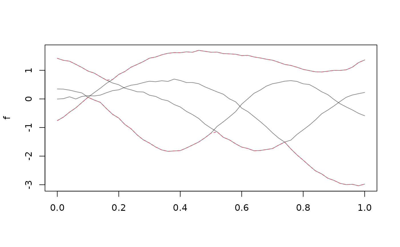
plot(f, points = FALSE)
lines(range(f), col = 2, lty = 2)


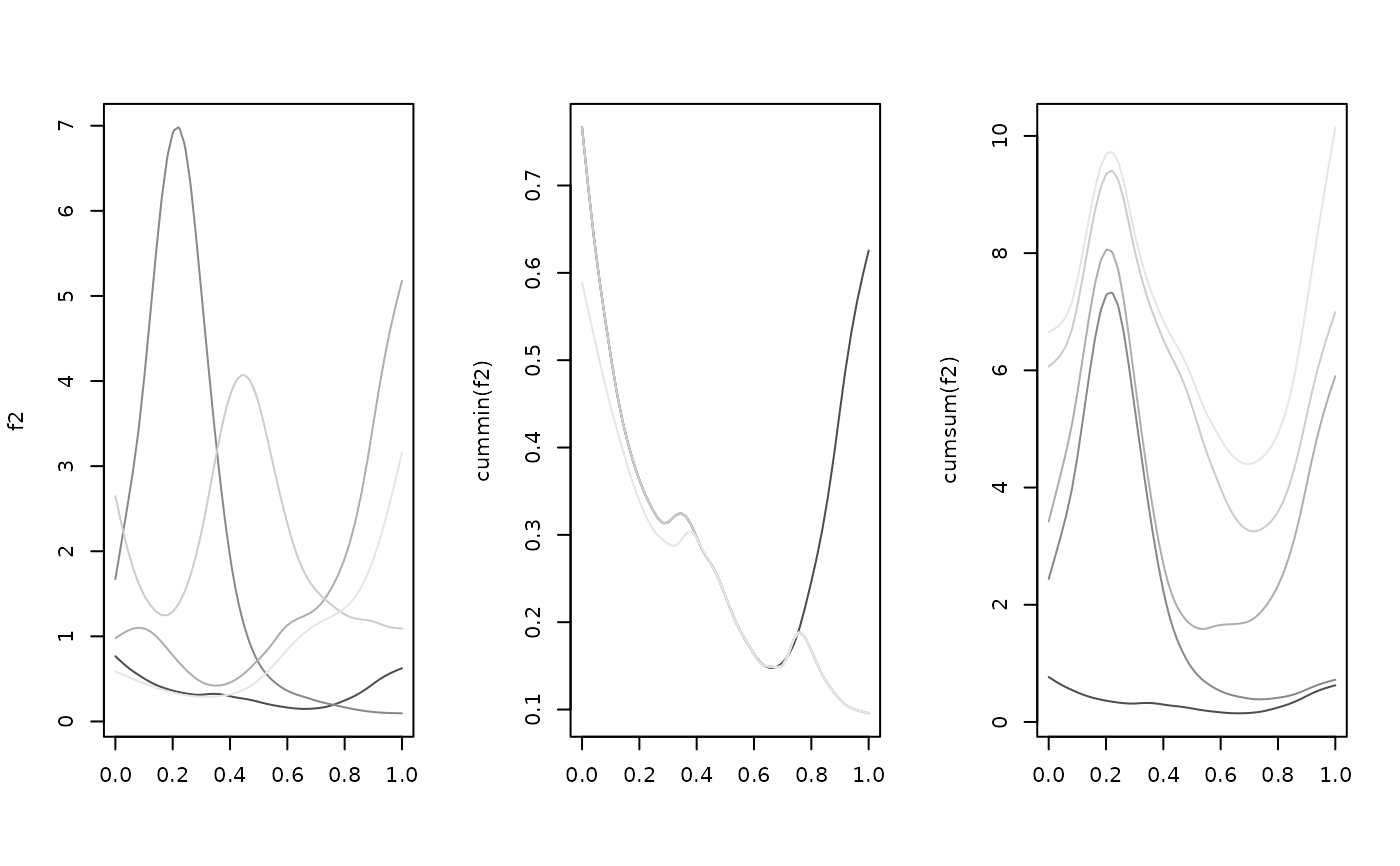
f2 <- tf_rgp(5) |> exp() |> tfb(k = 25)
#> Percentage of input data variability preserved in basis representation
#> (per functional observation, approximate):
#> Min. 1st Qu.  Median Mean 3rd Qu.  Max.
#> 99.70 99.80 99.90 99.86 99.90 100.00
layout(t(1:3))
plot(f2, col = gray.colors(5))
plot(cummin(f2), col = gray.colors(5))
plot(cumsum(f2), col = gray.colors(5))


# ?tf_integrate for integrals, ?tf_fwise for scalar summaries of each function